
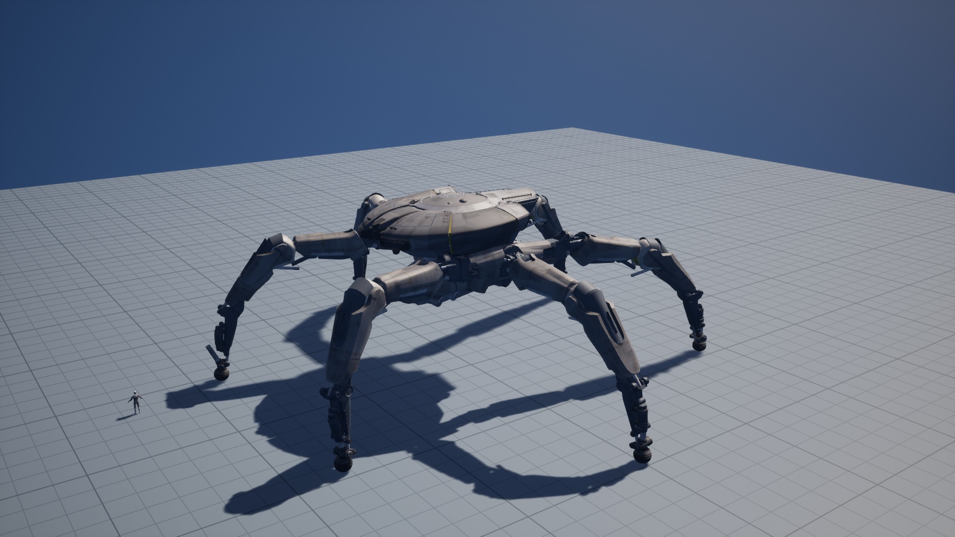
This series starts with robots and explores how procedural animation in Unreal Engine can support large creatures and different types of smaller creatures.
The first articles follow one multi-legged robot. This article covers gait, terrain contact, and physics-based control. The next looks at animation assets and their integration into UE. The third follows the handoff between locomotion, a stable stance, and an attack. Later articles will examine how much of this approach carries over to smaller creatures with different builds and skeletons. The implementation shown here is for the giant multi-legged robot.
When the giant robot in a third-person shooter stomps, the striking foot descends while the other legs support a moving body. In our Unreal Engine implementation, each foot has a separate rigid body for contact and force response, called a foot proxy. Inverse kinematics (IK) solves the visible leg chain from the body transform and the measured sole position. Even when the sole trajectory is continuous, the knee or ankle can exceed its frame-to-frame rotation limit on the next step. The controller predicts that physics state before the step and brakes the striking foot when needed.
For the giant multi-legged robot in this article, animation curves provide target trajectories for the body and striking foot. At runtime, terrain queries and physical contact inform foot targets, and IK solves the visible skeletal pose. The following sections trace how target generation, physics stepping, and pose solving exchange state, then examine how the controller preserves joint rotation continuity as the striking foot descends.
Contents
- Foot Trajectories, the Skeleton, and Physics Proxies
- UE Runtime Scheduling and Skeletal Pose Writes
- Support Anchors and Swing Trajectories
- Leg Geometry and Foot Reachability
- Frame-to-Frame Continuity of Knee and Ankle Poses
- Terrain Replay and Physical Ramp Entry
- Starts, Stops, and Turns on Flat Ground
- Body Force Control, Foot Actuators, and Contact Anchors
- Foot-State Prediction and IK Continuity Constraints During a Stomp Attack
- Sole Orientation and Terrain Coverage
- Source Code and Measurement Index
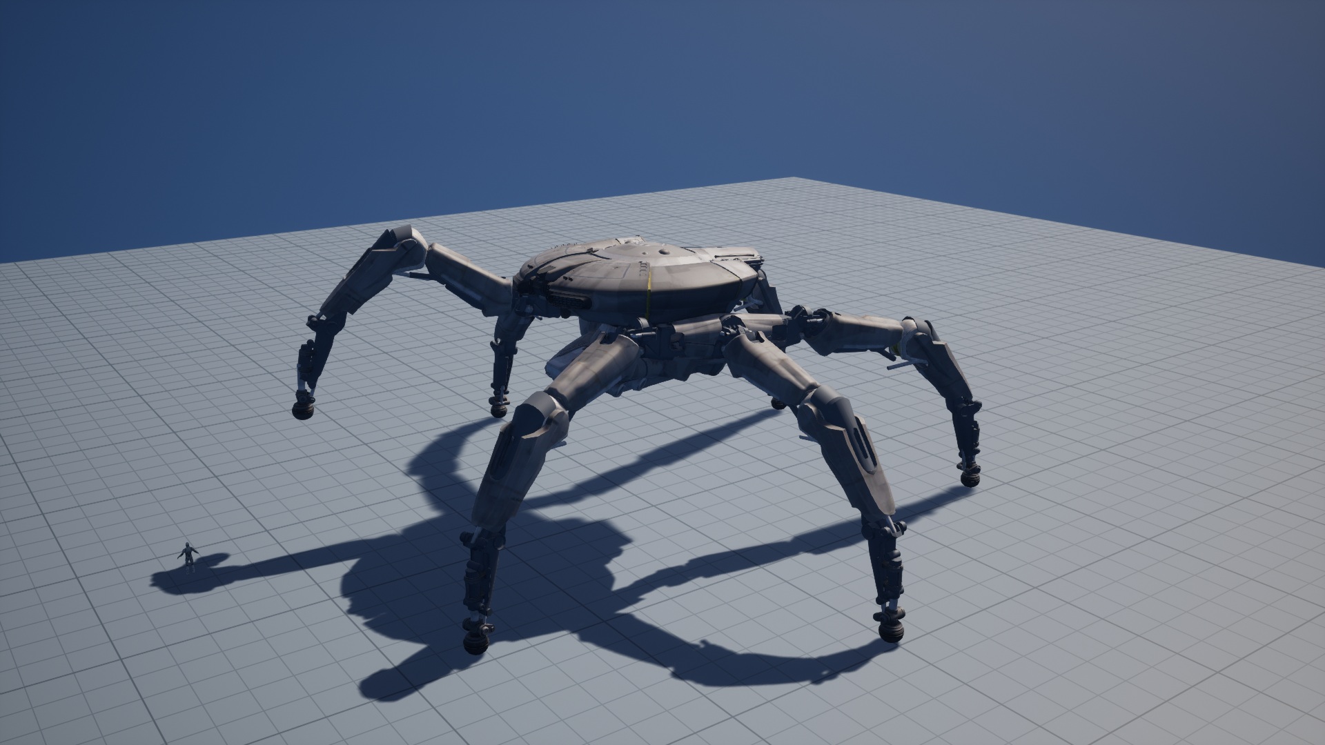
A kinematic replay solves the skeleton against planned footholds. The force-controlled runtime instead reads the sole position after physics advances, then solves the skeleton against that measurement. Starts, stops, and ramp entry show how these layers interact. The stomp adds a constraint on how much a joint may rotate in the next step. Part 2 covers animation assets and their integration into UE. Part 3 follows stable-stance observations into attack scheduling.
Foot Trajectories, the Skeleton, and Physics Proxies
A kinematic replay can start with a body pose and six sole targets, then solve for joint transforms. Terrain elevation affects the footholds, and the placement of the supporting feet constrains body motion. In the force-controlled test, a controller submits targets to one body and six foot proxies. After physics advances, it reads back their positions, rotations, and contacts. Driving the visible skeleton directly from the plan would hide the proxies’ tracking error.
| Data | Data source and use | What it establishes |
|---|---|---|
| Desired body pose and sole targets | Generated by the action or gait for the replay or controller | The desired motion and planned support transitions |
| Measured body and feet | Produced by physics for feedback and pose solving | Where the proxies moved and which feet made contact |
| Validated skeletal pose | Produced by IK and continuity checks for the skeletal component | Whether the skeleton follows the measurements and maintains a continuous pose |
| Support state | Derived from contact and handoff conditions for the controller or attack eligibility checks | When a foot can provide support and when the body is stable |
Let pGoal be the planned sole position, pMeasured the physics readback, and pFK the sole position reconstructed by forward kinematics (FK) from the solved bones. Express all three in the same coordinate space.
eTrack = ‖pMeasured − pGoal‖
eIK    = ‖pFK − pMeasured‖
A large eTrack and small eIK mean the skeleton follows the physical proxy closely while the proxy departs from the plan. Frame-to-frame rotation is a separate check because different knee and ankle configurations can reproduce the same sole position. Read the transforms back from the skeletal mesh component after writing the pose.
UE Runtime Scheduling and Skeletal Pose Writes
The host entry point for the start-and-stop footage is Locomotion.step(speed, turn). The first call records the origin of the game clock. Subsequent calls subtract that origin to produce the relative time passed to the planner. Forward speed and yaw rate are separate inputs. This demonstration interface accepts a forward request from 0 to 50 cm/s and a turn request with magnitude at most 1.5°/s. The later 100 cm/s cadence test used a different configuration.
At initialization, the host creates one body proxy and six foot proxies, enumerates their mesh components, and checks their count and mass distribution. This check applies to physics components. The visible mesh has full leg chains, while six discrete foot proxies provide rigid-body feedback. The solver determines the knee and ankle configurations. The UE proxies supply contact and inertia.
Gait planning and IK based on physics readback run in separate worker processes. The planner generates targets from the movement command, the latest body pose, and the foot observations. It can request a terrain query from the host, which performs the raycast and returns the result. The IK worker receives the measured body and feet along with the planned phase and target. A single leg can therefore carry both a target and a measured position.
The host keeps at most one outstanding planning request. An update services the message queue, answers terrain queries, replaces latest with any completed plan, and reads physics. When no request is pending, it submits the current readback, motion command, previous knee plane, and ankle offset. Pose solving starts once a plan is available and can combine the latest completed plan with the current measurement. The log records the plan’s sample time in planner_time and whether a request is outstanding in planning_pending.
After measured-foot IK returns, the host reconstructs auxiliary bones from their parent poses and local transforms. It then submits the current proxy targets. The visible skeleton uses the state read before that submission. The effect of the new targets appears in a later physics readback. If IK returns an error, the normal update terminates before target submission and retains the request and error information.
The stomp reuses the proxies and measured-pose solver through an external target entry point. On entry, a previously solved pose is available and the host temporarily disables solver sleeping. A body-to-target distance above 0.05 cm also triggers an explicit wake request. Action-generated body and foot targets replace ordinary gait targets while the gait clock is paused. On exit, the host accounts for the paused time and restores the original sleep configuration. Cleanup records are the evidence for successful restoration.
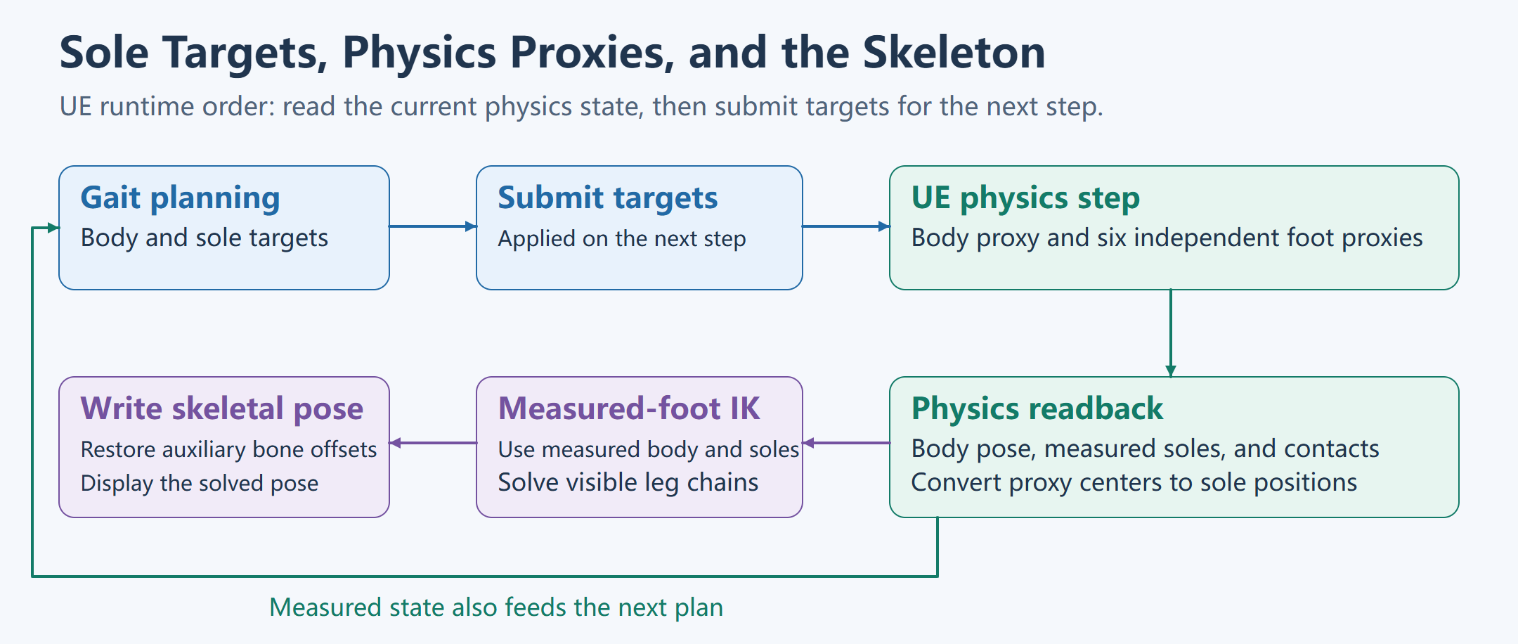
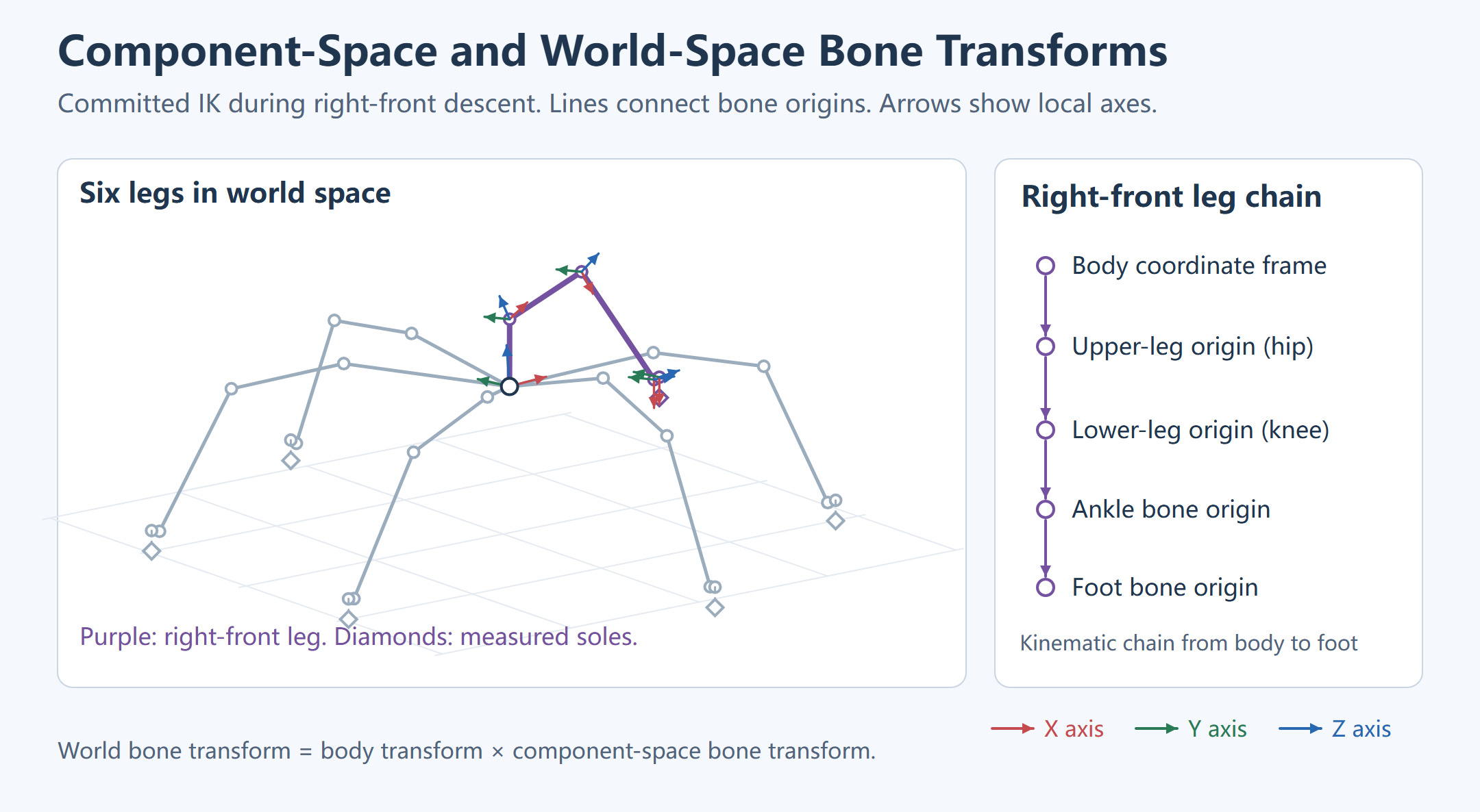
Rigid-Body Transforms and Sole Coordinates
The foot proxy’s reported position is the center of its component. The IK sole point subtracts the local offset (0, 0, 10 cm) after rotating it by the proxy quaternion. The offset therefore follows foot orientation. The ground query supplies a point on the contact plane and its normal. The host uses a dot product to obtain the signed normal distance and projects the sole onto the plane. The contact point, sole point, and proxy center have separate fields.
The host decomposes velocity into the normal component dot(v,n) and tangential speed ‖v − dot(v,n)n‖. Stable-foot observation requires valid native contact, active support, an active anchor, tangential speed ≤0.001 cm/s, and absolute normal speed ≤0.01 cm/s. Collision events or substep logs are needed to identify the first collision.
Contact Constraints and Stable-Stance Detection
| State | What the record confirms |
|---|---|
| Native contact | A valid physics contact |
| Active support | Native contact is valid and the current plan designates the foot as a support |
| Active anchor | The physics anchor is active and can constrain tangential motion |
| Stable-foot observation | The preceding conditions hold and the foot meets the tangential and normal speed limits |
| Whole-body stability candidate | All six feet are stable and the body meets the linear and angular speed limits |
The stomp’s load-bearing verification frame is the checkpoint selected in the delivery record. An earlier valid contact sample can be identified separately in the same run.
The locomotion host flags a whole-body stability candidate when all six feet are stable, body speed is below 0.1 cm/s, and angular speed is below 0.005 rad/s. Attack coordination then checks sample freshness and how long the condition has held.
Runtime Clocks and Sample Alignment
| Clock | Origin | Use |
|---|---|---|
| Scenario time | Start of the scripted scenario | Locate scripted walk, stop, and turn commands |
| Game clock | UE game time | Check when the host issued a command |
| Gait phase clock | Time accumulated by the planner, which can pause while waiting for contact | Determine stance or swing |
Plan sample time (planner_time) |
Timestamp carried by the latest completed asynchronous planning request | Compare plan time with the current physics readback |
| Stomp action time | Start of the committed stomp, at zero | Align curve progress, braking commands, and video frames |
| Stomp physics readback time | Clock for the physics recording, including pre-action operation | Pair rigid-body state with the corresponding action sample |
Support Anchors and Swing Trajectories

A stance foot can hold a world-space anchor. As the body advances, that fixed point moves backward in body space. Holding a constant body-local point instead would translate the foot with the body and produce sliding. A swing foot needs a lift-off point, a new foothold, and a phase value. The travel direction determines the plane of the swing, and the current reference transform converts each target for the leg solver.
The following equations illustrate that separation. Runtime modules handle curve sampling, leg group scheduling, and support transitions.
stance:  footWorld = supportAnchorWorld
swing:   footWorld = lerp(liftOffWorld, landingWorld, s)
                    + height(s) × groundUp
IK:      footInBody = inverse(T_body) · footWorld
At s = 1, the trajectory has reached its planned endpoint. The proxy may still be approaching it, or may have made contact without settling. Physics observations determine the transition into support.
Ramps and steps require separate foothold and swing-path checks. A reachable target on the upper surface leaves open the possibility of colliding with the riser during swing. Body motion can also bring another support leg to its reach limit. Terrain queries identify the surface, foothold validation checks the target, and path samples check swing clearance.
Stance Transitions and Contact Gating
A planted anchor stays in world space. When a leg enters swing, the planned sole target comes from the trajectory, while the measured sole still comes from physics. If the foot approaches its target without a confirmed contact, the planner waits so that the next group does not lift before replacement support is available.
The stomp tests use two contact criteria. Free-flight interval selection uses native contact and sole clearance. A support handoff additionally requires active support, an active anchor, and a stable observation. The first criterion excludes collision from the prediction test. The second excludes contacts that have yet to settle. The ramp figure shows the contact distribution in a single sample. The stomp trace also records the striking foot’s load-bearing checkpoint.
Anchor drift over the stance interval is the relevant measure for foot sliding. Handing the body to a combat action also requires body linear and angular speed. A successful single-frame anchor check supplies only the current foot position.
Establishing a Gait Baseline with a Community Hexapod Model
An early experiment used Carlo Romeo’s ARC_RL as a runnable hexapod baseline. The simplified model and MuJoCo environment came from the community project. The experiment ran the repository’s scripted phase controller and PD controller to generate motor commands. ARC_RL source
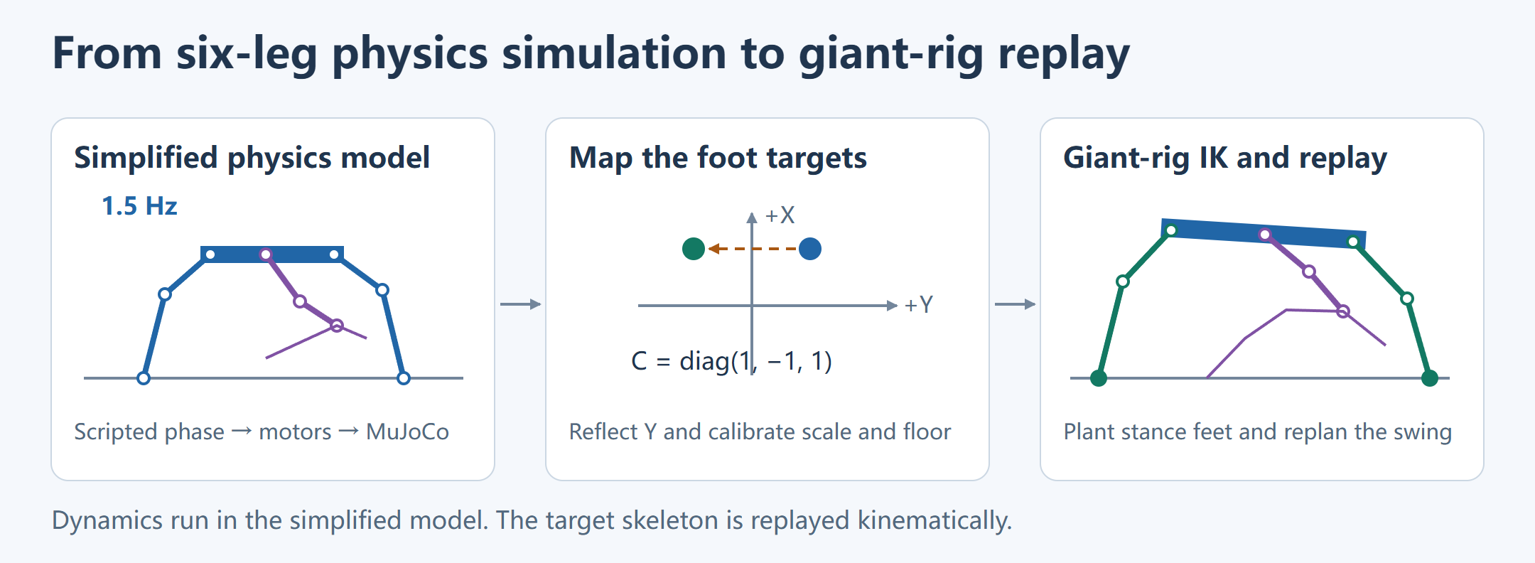
Run the simplified model. The controller divides the six legs into two tripods with a half-cycle phase offset. Each leg gets hip, knee, and ankle targets according to its stance or swing phase. PD control uses those targets, measured joint angles, and joint velocities to produce normalized actuator commands clamped to [−1, 1]. The slow, medium, and fast presets share a frequency of 1.5 Hz and vary their stance duty factor and joint amplitudes. Over 10 seconds per preset, the simplified root moved about 3.57, 4.73, and 5.66 m net along X, respectively.
Map the trajectory to the target skeleton. The local bridge reads the medium preset’s root translation and six world-space foot positions. The source model uses +Y for its left side, while the target skeleton uses −Y, so the position mapping uses C = diag(1, −1, 1). The median of the six ratios between target and source reference foot radii gives a scale of about 1,714.29 cm per source-model meter. The lowest sampled position of each foot sets its floor baseline. The bridge holds the body upright and passes the mapped body and foot positions to continuous IK. Across the 300 accepted frames, the largest frame-to-frame leg rotation was about 4.827°. The lowest collision hull point was about 0.48 cm below the floor, within the experiment’s 0.75 cm geometry tolerance.
Replan at giant scale. A later demo capped local speed at 200 cm/s and slowed the body path and gait clock together, yielding a cycle of about 4.83 seconds. Stance feet use fixed world anchors, and the local planner generates new swing trajectories. The 20-second UE clip below shows this stage as a kinematic replay with the original mesh materials. The later tests of starting, stopping, turning, and ramp contact use their own physics records.
Gait Phase, Foothold Planning, and the Swing Path
ForceGaitBridge and OnlineGait document the reference low-speed gait. Hashes of the underlying dependencies have not been matched to the flat-ground footage, whose direct evidence is the recorded video, command events, and verified host code.
L and R denote robot left and right, while 01, 02, and 03 denote front, middle, and rear. The stomp strikes with the right-front foot, R_01. The reference gait offsets L_01, R_02, and L_03 by half a cycle. The group containing R_01, L_02, and R_03 starts at zero offset. The fractional part of gaitClock / cycle + offset gives the leg phase. The bridge overrides the gait class’s 2 s cycle with 4 s. At a stance fraction of 0.6, each leg nominally spends 2.4 s in stance and 1.6 s in swing. The groups are offset by 2 s, so the nominal overlap at a transition is 0.4 s. Six-foot stable contact is still determined by observation.

Crossing the phase boundary alone does not initiate swing. The reference implementation considers both requested and internal forward and turn speeds, using foot scale to express turning on a comparable tangential scale. A foot already in stance holds position below the threshold, while a foothold safety stop is latched, or while the system waits for contact. Turning at zero forward speed can still initiate steps subject to the same support and foothold checks. These conditions apply to the local gait.
At swing entry, the planner estimates the end of swing and the midpoint of the next stance phase. It transforms the foot’s nominal local position using the predicted body position and heading at that midpoint to get the ground query point. This leaves reach available on either side of the next support interval. It adds the horizontal error between the actual and reference body positions to the forecast. The ground hit, sole clearance, and normal define the candidate endpoint. Foothold validation uses the body pose predicted for touchdown.
The reference code checks clearance at 39 interior swing samples. It queries terrain along the horizontal interpolation and solves for a lift amplitude. If pBaseZ is the baseline height at a sample and g(u) is the lift profile, the sample requires at least (surfaceZ + 2g(u) − pBaseZ) / g(u). The largest requirement is compared with a 20 cm floor. As g(u) approaches zero at either endpoint, samples run from 0.025 to 0.975. The lift-off anchor and landing target handle the endpoints. Discrete terrain samples do not establish continuous clearance against arbitrary obstacles.
Each swing sample clamps (u − 0.15) / 0.7 to [0, 1] before applying an easing function. The horizontal position remains at the start for the first 15% and at the endpoint for the last 15%. The vertical channel adds lift × g(u). Surface normals are interpolated and normalized, and heading is updated from the same progress. The foot can lift before moving horizontally, then descend near the foothold. Foothold validation, tracking, and the support handoff still determine the runtime result.

If swing reaches its endpoint before contact is confirmed, the reference gait retains swing, fixes progress at 1, and searches a short distance downward along the endpoint normal. The search starts when the wait begins and is capped at 3 cm. The motion interface receives zero forward and turn inputs while the planner holds the previous horizontal reference and heading and pauses the phase clock. Once contact is confirmed, the measured sole becomes the new world-space anchor, followed by a 0.3 s contact-settling interval. In this implementation, settling begins at the measured position, so a visible slide is not an expected part of that phase. If foothold validation fails, the support foot remains at its previous anchor and the safety latch suspends new swings.
Leg Geometry and Foot Reachability
The stomp diagnostic measures the actual reference skeleton with the Mesh root aligned to the Actor and uniform scale set to 1. Summing the segment lengths from the hip through the lower leg, ankle, foot, and sole gives a triangle-inequality bound.
Lmax = Σ length(segment)
d = length(soleTarget − hip)
d ≤ Lmax
A target beyond this distance is unreachable under any joint rotation. With a fixed candidate contact plane and vertical separation dz, the horizontal radius is at most sqrt(Lmax² − dz²) for |dz| ≤ Lmax. Passing the distance test still leaves knee direction, ankle alignment, joint limits, other legs, and the ground to consider.
At about 1.53 s in one diagnostic, the requested distance for the left-rear support leg L_03 was 1,903.016 cm. Its reference chain length was about 1,849.765 cm, an excess of approximately 53.25 cm. The same distance computed from the measured body and sole was about 180.10 cm below the limit. The first value checks the requested body pose against the anchor, while the second checks the physical configuration that actually occurred. The other two left legs showed smaller violations. This diagnosis applies to the test inputs.
Reachable-Set Intersection Across the Support Interval
A stance anchor must stay reachable throughout its support interval. Project each frame’s hip position onto the contact plane and compute a horizontal radius from the vertical separation. A candidate lies in the intersection of the resulting disks. A vertical separation beyond the chain length leaves that frame with no feasible disk. This geometric test uses only body targets and segment lengths, so it can precede the more expensive joint search.
The stomp preparation planner further checks joint limits, self-contact, and FK reconstruction. The logged inward search spans 0–200 cm in 10 cm increments. Static ankle seeds are sampled within ±15° in 3° increments before the existing clearance checks. The three left anchors moved by approximately 105.00, 134.35, and 181.60 cm in local UE scale. The right middle and rear feet retained their positions and the same foot was selected to strike. This record checks per-leg candidates. Joint feasibility across the combined leg trajectories requires a separate test.
A physical preparation run adjusted support anchors one leg at a time and retained at least five observed contacts. The three resulting anchor errors were about 0.101, 0.079, and 0.050 cm. These footholds passed the preparation check, yet the action reached a frame-to-frame joint difference of 5.735° at about 1.80 s. Continuity depends on the actual body and striking foot throughout the action as well as the initial footholds.
Frame-to-Frame Continuity of Knee and Ankle Poses
Multiple joint configurations can reach the same sole position. In a two-segment leg, the knee lies on a circle when the root and endpoint are fixed. The knee plane sets the bend direction. Ankle and sole orientation constraints can redistribute rotation across adjacent joints. Minimizing a single frame’s foot residual can select a different configuration on the next frame.

The measured worker composes each bone’s component-space orientation with the body rotation. For unit quaternions, the absolute dot product makes the comparison invariant to the equivalent signs q and −q.
deltaAngle = 2 × acos(clamp(abs(dot(qPrevious, qCandidate)), 0, 1))
The formula yields radians. Compare it with the 5° limit in consistent units. The logged metric uses the previous committed pose as the reference. A candidate must satisfy both sole geometry and frame-to-frame rotation. Smoothing the final animation can delay visible touchdown or keep the bones interpolating after the foot is already loaded. The stomp instead checks continuity against the predicted physical state.
A discrete continuity search can be represented as a layered graph. Layer k contains the knee-plane and ankle-offset candidates at time k. Adjacent candidates have an edge if their frame-to-frame rotation passes the limit. Individually valid frames and even individual edges can exist without a connected path over the action.
The preparation run provides a concrete example. The R_01 transition between frames 54 and 55 failed continuity, with 470 candidates in each frame. An exhaustive comparison on the recorded knee-plane and ankle-offset grid found a minimum worst-joint rotation of about 5.522°, above the 5° limit. The grid search holds the physics input fixed. Enlarging the grid adds pose candidates, while braking changes the measured sole input for the following frame.
Terrain Replay and Physical Ramp Entry

A uniform slope is useful for testing the ground normal and body height. An 80 cm step exposes conflicts between the lift path and a vertical riser. Roof transitions require different elevations for front and rear support without moving every foot onto the higher surface at once. The archived slope, step, and roof clips show solved poses, swing paths, and support transitions in kinematic replay.
A separate physics run advanced from flat ground until the front feet contacted the ramp. The body traveled approximately 15.01 m, rose about 65.05 cm, and reached a peak adjacent-frame joint rotation of about 0.600°. Travel includes the flat approach. The run covers ramp entry.


Both front feet touched the 10° slope while the middle and rear feet remained on level ground. The measured front sole heights were approximately 188.6 cm and 171.8 cm. The surface normals confirm the distinction between the ramp and the flat approach. All six contact flags were true at this sample. Contact transitions over time require the continuous recording and per-step log.
The front feet differ by about 95.12 cm along X, the slope direction in the record. At 10°, the expected height difference is 95.12 × tan(10°) = 16.77 cm, which agrees with the measured difference.
The planned and measured sole coordinates coincide in this sample. The plan comes from the step’s actuator target and contact comes from a separate readback field. Joint actuator error and the load carried by each foot would require independent measurements.
Starts, Stops, and Turns on Flat Ground

The start-and-stop run requests 50 cm/s. Starting requires support, and the body acceleration depends on the actuators and contacts. After the request returns to zero, swing feet still complete their landings and residual angular velocity must decay. Measured body orientation establishes the turning result. Combat coordination reads the measured contacts and body velocities.
The turn recording shows two cases. In-place turning changes support placement. Turning while walking combines yaw with the gait. The body orientation in the recording establishes what moved, and the command log establishes the requested turn.
A separate cadence comparison requested 100 cm/s in both runs and retained normal playback speed. The 2 s cycle candidate increased measured mean speed from about 38.05 to 53.54 cm/s over the same window, a gain of about 40.7%. This result belongs to the cadence comparison. Isolating the contribution of shorter waits, shorter swings, or body acceleration would require aligning commands, phase transitions, and measured speed.
The start-and-stop script scheduled walk, stop, walk, and stop at about 2, 13, 22, and 26 s. The first command was issued at game time 2.033 s. Scenario time locates a segment, and the game clock identifies command delivery. The turn script requests a yaw rate of magnitude 0.9°/s, alternating direction over 0–10, 10–18, 18–28, and 28–37 s before returning to zero. A walk request arrives near 19 s, so the recording includes both in-place and moving turns. Contact waits, command filtering, and physical response affect actual yaw.
The control interface distinguishes starting, walking, turning, braking, swing-foot recovery, and stopped. It evaluates the current command and internal velocity separately. A turn request or residual turn speed can keep it in the turning state while forward velocity is nonzero. After the command is withdrawn, high residual speed keeps it in braking. As speed falls, unfinished swings or changes in support height keep it in recovery. Physical handoff still checks all six feet and body velocity, so stop input, stopped state, and attack readiness are distinct events.
The reference gait averages surface heights for feet in stance or contact settling. Position and velocity feedback generate a desired acceleration capped at ±20 cm/s². Acceleration changes are limited to 30 cm/s² per second. The old and new acceleration are averaged to update velocity, then the old and new velocity are averaged to update height. Velocity has a separate ±30 cm/s limit. Vertical adjustment can continue after horizontal motion stops. This smooths the planned target before the body proxy applies its own limits and contact constraints.
Start-and-Stop Commands and Body Speed Statistics
Compare requested and measured speed over the same window. Two 100 cm/s commands can produce different means when acceleration, support transitions, or swing-foot recovery take different amounts of time. The cadence test gains approximately 15.49 cm/s over a 38.05 cm/s baseline, about 40.7%. The mean does not describe the speed within individual swings.
To diagnose turning, align the requested yaw rate, measured body yaw, and contact flags. If the recording shows little rotation, check command delivery, angular velocity at the proxy, and pose publication. The handoff includes the scenario schedule and summary. It does not include per-step measured yaw for the turn clip.
Body Force Control, Foot Actuators, and Contact Anchors
The native calculation below is based on the retained QueenForceRig.cpp reference. The final stomp provides same-run mass, configuration, and physics readback. The retained C++ has not been matched byte-for-byte to the recording binary. The reference explains the controller structure, and the same-run output establishes measured values.
Body Position and Orientation Servos
The stomp log records a 6,000 kg body and six 800 kg foot proxies. The contact cache window is approximately 0.05 s. The solver’s maximum substep duration is about 0.001389 s, with a configured cap of 512 substeps. The 30 fps action sampling rate is separate from the internal solver. The free-flight prediction test used 25 substeps in the recorded case. The actuator calculates gains from the supplied step duration dt.
pole = exp(−ω × dt)
kp = (1 − pole)² / dt²
kd = (3 − 2 × pole − pole²) / (2 × dt)

aRequest = kp × (pTarget − pActual)
         + kd × (vTarget − vActual)
         + aFeedForward
The body position servo uses ω = 4 and limits the magnitude of the combined acceleration to 600 cm/s². A large vertical request leaves less horizontal capacity. The reference implementation initializes gravity loading after at least three valid support contacts. With support available, it multiplies mass by requested acceleration plus gravity compensation to compute body force. Loss of all support removes that compensation.
The reference controller caps tangential body force at 0.25 times the positive vertical force and scales down the horizontal vector if it exceeds that budget. Each foot has a configured friction coefficient of 0.5 in the stomp readback. The first value limits controller demand. The second configures foot contact. A slope limit cannot be inferred from either alone.
Orientation tracking uses the relative rotation and the difference between requested and measured angular velocity. The reference code transforms inertia into world space and uses angular acceleration to compute torque. The torque budget depends on the mean distance of supporting feet from their center. A tighter support footprint gives less torque budget for the same support force. The predictor sets roll and pitch inertia to 0.625 times the reported yaw inertia for this box proxy. A complete art mesh would have a different inertia model.
Support Reactions and Torque Distribution
With at least three supporting feet, the reference controller solves for a vector a. If foot i is at r_i relative to the support center, its torque-related force is a × r_i. Summing the moments gives:
W = Σ(‖r_i‖² I − r_i r_iᵀ) + 10⁻⁵ I
a = W⁻¹ τ
F_i = F_body / contactCount + a × r_i
I is the identity matrix and the small diagonal term regularizes the solve. The foot proxies receive the opposing forces and transfer the load through contact. With fewer than three supporting feet, the reference branch clears the body’s support torque. Orientation drives also introduce reaction torques. Turning can be checked by comparing contact distribution, torque demand, and measured yaw.
The foot actuator branches on planned phase. The stance branch uses ω = 5 for position and velocity feedback, projects its force onto the plane defined by the foot’s target orientation, and caps force at foot mass times 1,000 cm/s². The swing branch uses ω = 8 and includes target velocity, feed-forward acceleration, and gravity compensation. It clips the result to the foot’s swing acceleration cap. Both branches compare proxy centers, so the sole target is converted using the rotated 10 cm offset. For the first stomp braking step, the same-run R_01 packet sets the swing cap to 30,000 cm/s². The total actuator output remains subject to that cap after feed-forward correction.
The contact cache evaluates time since contact and the sole’s distance from the contact plane. A valid contact and a planned support flag jointly enable support for the step. Anchor handling evaluates the sum of actuator force, support reaction, and gravity. The host then checks anchor state and foot velocity to determine whether support has settled.
Foot-State Prediction and IK Continuity Constraints During a Stomp Attack
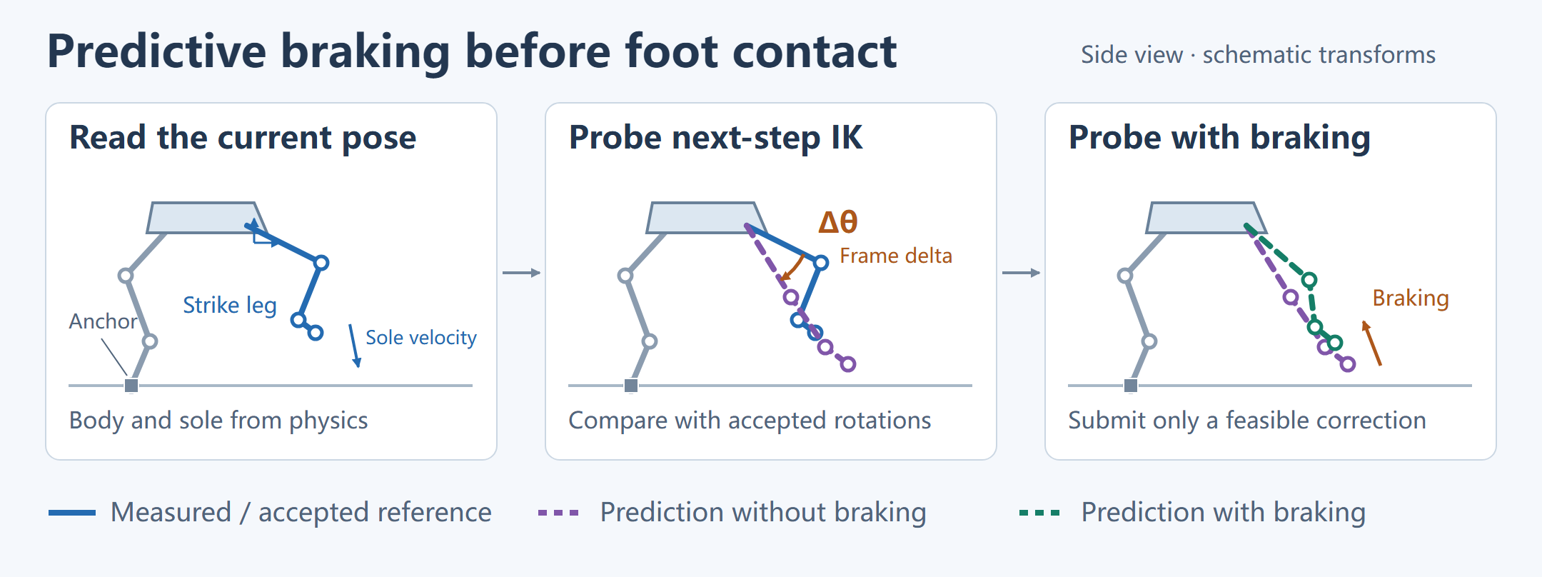
The stomp curve supplies an absolute body-height target. With world-space stance anchors fixed, raising the body can put the hip-to-sole distance outside the reachable set. The initial stance therefore reserves extension for the support legs. The preparation test checks the initial footholds. Joint rotation continuity during descent requires a separate check.
The 30 Hz test also exposed an integration issue. When a velocity breakpoint occurs inside a step, sampling instantaneous acceleration at the start and holding it for the entire step makes the velocity change dependent on sampling phase. In a separate integration check, a breakpoint should have produced 60 cm/s of velocity change. The old hold yielded approximately 400 cm/s or nearly zero depending on phase. The correction recovered about 60 cm/s at all three tested phases. It preserves the step integral Δv = ∫a(t)dt and uses Δv / Δt as the equivalent held acceleration. This test verifies the discrete correction independently of the UE physics run.
Stomp Animation Curve Sampling and Actuator Target Generation
The test takes its stomp curves from the Animation Repository and its action and recovery durations from the ability asset. The adapter samples these curves on the action clock to produce body transforms, striking-foot positions, and actuator feed-forward targets. The source action and recovery each last 2 s. Progress is clamp(t, 0, 4) / 2, so recovery samples the interval from 1 to 2. Capping progress at 1 would hold the main action’s final sample throughout recovery. The local adapter follows the reference task’s ownership convention. The ability asset alone does not establish the original task lifecycle.
For horizontal translation, the adapter subtracts the initial curve value from the current one, scales by RefPoseBodyHeight, rotates into the action heading, and adds the result to the prepared body position. It writes Z separately as the initial striking foothold height plus the scaled absolute curve height. Treating Z as an offset from the initial curve value would change the starting pose and available extension. Body orientation composes the local curve rotation with the parked reference pose.
For the striking foot, the adapter multiplies the two horizontal channels by a local factor of 150, clamps height to a nonnegative value, rotates the vector by the action heading, and adds it to the foot anchor. The other legs retain the prepared support anchors. A different character or mesh scale calls for checking that factor, the reference body height, and the leg-chain lengths separately.
The source action and recovery occupy 4 s. A local return controller takes over for approximately 2 s, blending the body and striking foot back to the parked reference. It adds 30 × sin(πf) cm of lift, with f the normalized return progress. The run waits until measured velocity, position error, and six-foot contact meet the settling criteria for 2 s. The finished clip includes action, recovery, return, and settling.
The adapter derives velocity and acceleration from position samples spaced by the servo’s hold interval. It samples around the center when possible and uses forward samples for acceleration near the start. Velocity and acceleration magnitudes are capped at 3,900 cm/s and 49,000 cm/s². These are feed-forward fields. The actuator subsequently combines tracking error, mass, and gravity compensation and applies its own output limit. The log distinguishes braking acceleration, the limited feed-forward input, and actual actuator output.
Servo Integration Correction and IK Continuity Verification
The servo comparison keeps position, rotation, phase, and timing inputs fixed. In the first 50 frames, both runs still accept poses. In that window, tracking root mean square (RMS) error falls from approximately 154.72 to 1.67 cm, and the peak falls from 279.68 to 4.87 cm. The full physics log includes diagnostic samples after the first rejection, when feedback continues with the last accepted pose. Across that longer window, RMS falls from approximately 145.35 to 3.15 cm and the peak from 404.94 to 9.03 cm. The latter pair describes full-window physics tracking.
Before the correction, the first IK rejection occurs near 1.667 s at 5.614°. After correction it occurs near 1.800 s at 5.617°. Improved proxy tracking leaves the first rejected pose above the 5° limit.
A separate initial-stance test took 166 frames to prepare. The body closed from about 400.35 cm away from the source initial target to about 0.000035 cm, with all six feet in contact at the end of preparation. The subsequent action used the original sample times and first failed near 1.800 s at about 5.322°. This test and the three-anchor repositioning test have separate records. Neither improved initialization nor better position tracking resolved the descent discontinuity on its own.
Finite differences of the source body targets gave peak requested speed and acceleration of about 725.68 cm/s and 5,595.70 cm/s². Eight samples exceeded the local 499 cm/s speed limit used in that comparison, and 44 exceeded the 600 cm/s² acceleration limit. This quantifies how quickly the request can move ahead of the proxy. It does not establish the original game’s force, mass, or stiffness or show that raising limits would restore continuity.
Another diagnostic froze measured feet and sample times and substituted only body translation, only rotation, or the complete transform. The variants still exceeded the rotation limit at about 5.124°, 5.757°, and 5.204° respectively. These offline substitutions isolate body input without changing the original recording.
Support-Leg Reach and the Body Height Ceiling
The disk intersection is an initial-stance test. During motion, the support leg’s actual ankle orientation changes with the body. BodySupportFeedback uses the accepted pose and measured sole, then removes the sole-to-foot and foot-to-ankle offsets to obtain the current ankle target. Its radius covers hip-to-knee and knee-to-ankle. The earlier hip-to-sole test uses a broader whole-chain bound.
For each observed contact with no planned swing, rotate the hip offset with the body. Use horizontal displacement dXY between hip and ankle to constrain body Z:
zLimit_i = ankleZ_i − hipOffsetZ_i + sqrt(r_i² − dXY_i²)
rawCeiling = min(zLimit_i)
The implementation rejects inputs at the horizontal reach radius and requires at least three usable support legs. If a future body target is available, it computes another ceiling for that pose and uses the lower of the current and future bounds. The forecast horizon is 0.5 s. A future horizontal target outside the radius fails explicitly. The vertical constraint preserves the original foothold anchors.
The controller estimates downward motion of the ceiling from successive bounds. Let closing be the body’s positive approach speed relative to the bound. It subtracts 0.05 cm, the next step’s approach distance, and a half-step-squared term based on 600 cm/s². It estimates stopping distance as closing² / (2 × 600). This allows the controller to reduce upward acceleration while geometric reach remains available.
The solver first evaluates the unconstrained body servo. If safe Z acceleration is lower, it constrains Z and assigns the remaining magnitude sqrt(600² − aZ²) to XY. The correction is written into body feed-forward acceleration. The source body position and action time remain reference inputs. A source target above the ceiling calls for checking approach speed and the applied correction before diagnosing tracking error.
Near 1.767 s, the left-rear support leg is the limiting case. Its current geometric ceiling is about 1,097.09 cm, with about 2.68 cm of discrete margin. Its future-pose ceiling is about 1,005.90 cm, giving an effective limit of 1,003.22 cm after the margin. The measured body is at 954.77 cm, while the source target is at 1,033.07 cm. The unconstrained servo already requests downward acceleration, so the logged support reaction correction is zero. The ceiling constrains the step’s control output while leaving the source curve available for comparison.
Body-Transform Substitution with Fixed Foot Inputs
This diagnostic takes measured body transform, measured soles, and the previous pose. It reproduces the failure with the original inputs, then substitutes translation, rotation, or both. The variants share foot trajectories, sample times, and initial pose. All three still produce frames above the angular limit. Body-transform correction alone does not remove the striking leg’s discontinuity.
Knee-Plane and Ankle-Offset Search in Continuous IK
The same rotation metric has three thresholds. A difference above 2.5° triggers a local search for a better IK solution. A predictive candidate must stay at or below 4.8°. An IK solution computed from actual physics state is rejected above 5°.
The measured worker first solves from actual body and foot proxy poses, then checks clearance. The final stomp worker searches redundant coordinates. For each upper leg, lower leg, ankle, and foot, it combines component-space bone rotation with body rotation and measures the maximum adjacent-frame difference across the six legs. A parent-local comparison alone would omit changes caused by body rotation.
When a leg exceeds 2.5°, the search alternates ankle-offset and knee-plane adjustments in the order ankle, knee, ankle, knee. It tests signed perturbations of increasing size, then refines around the selected offset. Each trial restores its starting knee-plane and solver state, reruns IK and clearance handling, and checks limits and same-leg collisions. A valid candidate replaces the original only when it reduces the leg’s maximum rotation difference. Planned sole and time step remain fixed during the search.
The complete solve then checks FK sole error, joint limits, same-leg collisions, and the 5° limit across all legs. Only a committed solve updates the previous pose. Prediction calls the same solver with hypothetical inputs and restores the previous pose, clock, and mutable state on exit. Both normal and exceptional paths compare the before-and-after state fingerprints.
Pre-Step Foot Prediction and Isolated IK Probes
The predictor runs before physics advances. With the swing foot in free flight and sufficient ground clearance, it uses measured state and actuator input to estimate the next proxy position. The predicted body and sole go to an isolated IK probe that checks maximum rotation relative to the previous committed pose. A candidate above the predictive limit can trigger a bounded braking correction in the current step.
A separate readback test compared 128 free-flight intervals against UE’s next recorded states and excluded 185 intervals at or near contact. Selection used native contact flags and 1 cm of clearance. Maximum sole-position difference was approximately 3.68 × 10⁻⁵ cm for these controlled free-flight inputs. Collision and contact solving were outside the comparison.
Read measured body and foot state
Predict the next proxy state during free flight
Probe IK and check the frame-to-frame rotation
Restore probe state
Submit the selected correction to physics if braking is required
Read the next measured state, solve, and publish the pose
Probe state and the committed runtime record are kept separate so that one candidate cannot change the starting point of the next. The final run records 163 probe packets and logs their restoration separately from submitted braking.
Search for Swing-Foot Braking Acceleration
Prediction requires the striking foot to be in free swing and the other five feet to have active support and fixed anchors. It skips a foot that is waiting for contact, already has a native contact flag, or is observed less than 1 cm above the surface. If the unbraked prediction drops below 1 cm, the free-flight check also exits. The model advances the proxies by one step. Contact impulses and anchor activation are resolved in the actual physics step.
The predictor computes body and striking-foot acceleration with the reference gains and limits. Starting from measured velocity, it uses a position coefficient of 0.5 × (1 + 1/N) for N substeps. Under constant acceleration, updating velocity before position gives the coefficient by summing 1 + 2 + … + N. For body rotation, angular velocity and estimated angular acceleration form a rotation vector, which is converted to a quaternion increment. Free-flight position and rotation were checked against recorded next states.
A braking candidate changes only striking-foot feed-forward acceleration. Its direction is opposite measured foot velocity. The candidate magnitude times that direction is added to the original feed-forward vector and limited to 49,000 cm/s². The predictor advances the modified packet once and sends the resulting body and sole to isolated IK. The candidate must solve without errors, stay at or below 4.8° of joint rotation, and keep FK error at or below 0.05 cm. The measured worker keeps its 5° rejection threshold.
The search tests zero braking first. If it fails, it tries 1,000, 3,000, 6,000, 12,000, 20,000, and 30,000 cm/s² until it finds a feasible upper endpoint. It then tests eight midpoints between the most recent failure and the feasible value. A pass tightens the upper bound, and a failure raises the lower bound. The search retains a packet already verified by the probe. It does not establish global monotonicity or a global minimum. If there is no feasible candidate, the caller records the failure and rejects the run.
| Action time at submission | Predicted max angle without braking | Selected braking (cm/s²) | Predicted angle with braking | Measured angle on the next frame |
|---|---|---|---|---|
| 1.767 s | 5.32160° | 12,187.50 | 4.79969° | 4.80017° |
| 1.800 s | 5.00781° | 4,664.06 | 4.79964° | 4.79955° |
| 1.833 s | 4.98022° | 3,867.19 | 4.79970° | 4.80022° |
In the first search, 12,000 cm/s² predicts about 4.80823°, within the committed 5° threshold but above the predictive margin. The first candidate within the margin is 20,000 cm/s², after which the search tightens toward a lower value. The third unbraked prediction already falls below 5° but still exceeds 4.8°. Each correction is recomputed from a fresh physics readback.
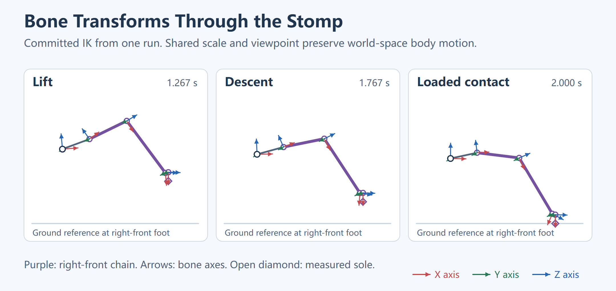
Aligning Braking, Contact, and Skeletal Pose
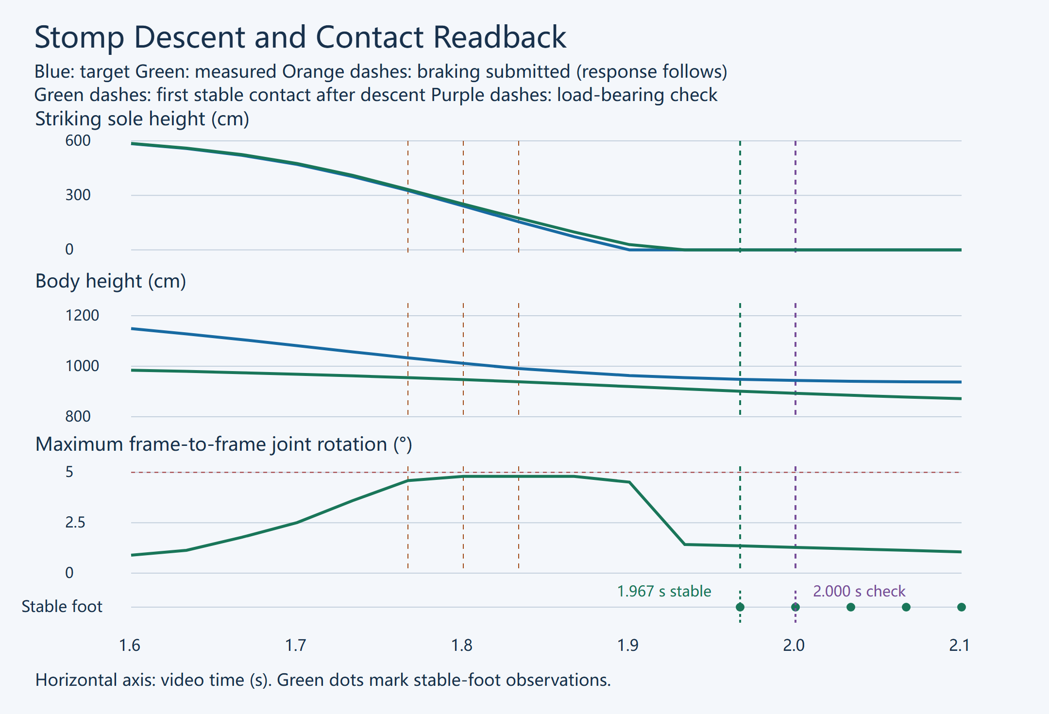
The start of the action corresponds to about 7.6 s in the physics log. Both clocks label the same sample from different origins. Command response is visible in later readbacks. All 314 action samples were aligned against the committed IK log using the body and six measured sole positions. The worker request timestamp is one sample, about 33.3 ms, ahead of the corresponding physics readback timestamp. The plot matches physical states directly without interpolating. Probe packets are logged separately. The 166 preparation samples affect the initial pose and stability and are outside the 314 recorded action samples.
At about 1.767 s, before the first braking command, the measured striking sole was about 331.91 cm high with vertical velocity of about −2,494.97 cm/s. The 326.36 cm target on that row was sent after readback. Near 1.900 s, the target had reached the ground while the measured sole was still about 28.86 cm above it. In the next sample, measured height was nearly zero, with contact, support, and anchor still false. Sole height, valid physics contact, and stable observation are distinct sample events.
At about 1.967 s, the first stable-foot observation after descent is recorded. Native contact, support, and anchor are valid, and all six stable-foot observations are true. The delivery record uses the later 2.000 s frame to verify load-bearing contact. Determining the first collision substep would require a finer-grained contact log.
Peak measured frame-to-frame rotation is approximately 4.80022° at 1.867 s. It lies slightly above the 4.8° prediction margin and within the committed 5° limit. The predictive margin applies to the trial estimate. Measured state and execution determine the committed result.
The final 30 Hz test records 314 frames and preserves the original desired curves and sample times. Maximum measured joint rotation is approximately 4.8002°, and maximum FK reconstruction error is about 0.000009 cm. End-of-recovery errors are approximately 0.000038 cm for body position and 0.0153 cm for foot position. These figures describe continuity, skeletal reconstruction, and recovery respectively. The three submitted corrections belong to this stomp run.
Sole Orientation and Terrain Coverage
The local sole-pose adapter preserves proxy rotation. Recovered class defaults include a 0.2 s landing-alignment window and orientation rate limits of 80°/s in motion and 360°/s in support. Runtime overrides may change these values. The local path still needs the source script’s airborne displacement lag and approach-to-contact orientation. Integration would require the actual planted and just-planted states, time to touchdown, the foot twist axis, and the ground-alignment transform.
An independent alignment replay retained recorded body and sole positions and recomputed only foot orientation. With the native runtime services unavailable, it derived the alignment countdown retrospectively from logged contacts and used local mesh clearance for sole height. The native twist query was unavailable. The complete leg replay still reached about 5.221° of joint discontinuity near 1.80 s. This bounds what orientation reconstruction alone achieves with the available inputs.
A fixed-clock test verified how the client reads an existing forced-step record. It converts time values to float32 on the original path, subtracts current interpolation time from step end time, and clamps the result to a nonnegative value. The test covers remaining-time calculation. Whether the stomp creates that record and when it writes it remain upstream questions.
Flat-ground starts and stops, turning, ramp entry, and the local stomp have separate records. The current physics controller still lacks continuous tests for reaching the ramp crest, descending it, or crossing roofs. The final stomp retains per-frame targets, measurements, and braking search results. Starts, stops, and turns have host code, command events, and footage from their respective runs, with no per-step physics readback. Some reference dependencies have yet to be matched to the recording binary.
Source Code and Measurement Index
| Question | Entry point or record |
|---|---|
| Flat-ground commands and worker scheduling | Verified host code and scenario events for the start-and-stop and turn runs. See Locomotion.observe and Locomotion.step |
| Foothold planning and contact waits | ForceGaitBridge, OnlineGait, and the control interface. The underlying dependencies are retained references |
| Stomp curves and actuator targets | source_recovery_stomp, the batch validation entry point, and same-run effective parameters |
| Braking candidates and synchronized physics and IK | guard_swing_joint_step, probe candidate records, and the 314 paired physics and committed IK samples |
| Body force control and foot actuation | QueenForceRig.cpp explains the reference algorithm. Same-run readback verifies final stomp mass, contacts, and forces |
1 thought on “Procedural Animation for Robots, Part 1: Gait and Physics-Based Control for a Giant Multi-Legged Robot”