
Contents
- Terrain Geometry, Zones, and Material Distribution
- Zone Meshes and Raster Coverage
- Slope, Noise, and Route Weights
- Weight Writes and Draw Order
- Class Selection and 32-Bit Packing
- Runtime Class Filtering and Material Blending
- Sand Textures and Surface Shading
- Carrying GPU Weights into Blender
- From Material Outputs to the Final Image
- Locating Differences in the Pipeline
- Reconstruction Scope and Remaining Inputs
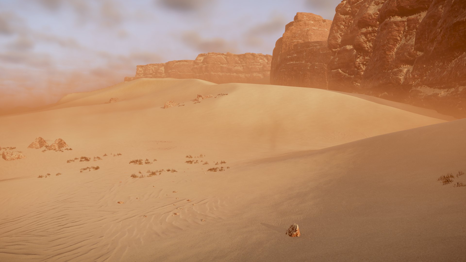
The ripples in the foreground fade across the slope. The darker slope on the right has a much finer grain. Both are part of the same heightfield, but their surface materials are distributed by a separate generation pipeline. Change the layer weights while keeping the terrain geometry fixed, and the ripples move to a different part of the slope.
In HD2’s Desert Sandy case, slope, noise, and route passes write to GPU weight buffers. A merge pass compresses the candidates at each location into a 32-bit material word. At runtime, the renderer reads neighboring material samples and computes opacity for each material draw. A single point on the sand lets us work through both representations before examining the ripples, lighting, and aerial perspective in Blender.
The archived game capture provides the final generated material data. Controlled replays use archived inputs, explicit starting conditions, and original GPU programs to reconstruct specific draws. Blender provides a separate check on the current texture bindings and rendered result. The three can be registered in world space. The historical draw order and resource bindings still depend on the records available for each experiment.
Terrain Geometry, Zones, and Material Distribution
Heightfields and Material Weights
A heightfield assigns an elevation to each horizontal position. It can supply the terrain geometry and the neighboring samples used to calculate slope. With the geometry held fixed, a change in material or weight changes the color and light response without moving the broad contours of the slope. A separate displacement test later in the article compares actual changes in vertex position.
A Zone is a spatial region in the generation configuration. It supplies the choice and extent of material draws, so different Zones can apply different rules to the same material. A point near a boundary may receive coverage from a neighboring draw mesh, or be modified later by a route or a raw material draw. The boundary on a Zone map and the continuously interpolated value at the shader input are separate observations.
Before merging, a pixel’s material distribution can be represented as a vector W=(w₀,…,w₃₁). Each component stores the accumulated value of one material class. The merge pass packs the selected classes and weights into a 32-bit word. Runtime processing uses neighboring samples and material inputs to form new candidates and opacities for the material draws that follow.
| Data | What it describes | Evidence used here |
|---|---|---|
| Height and property height | Terrain elevation and the input sampled for slope | Archived heightmap and the property-height resource declaration in the original shader |
| Zone and material draw mesh | The region in which a rule applies and its coverage near boundaries | Registered Zone data and controlled replay of the native mesh |
| Weight targets before merging | Which class channels a draw changes | Per-step 32-channel arrays and maps on a 512² grid |
| Generated material map | The classes and weights retained at each output texel | Original 4096² capture and tests of the original merge shader |
| Runtime material map | Whether a material draw contributes at a pixel, and with what opacity | Original consumer instructions, controlled GPU output, and world-space registration |
| Source textures and rendered material | How color, ripples, and highlights appear on the surface | Original texture channels and single-layer and blended Blender renders |
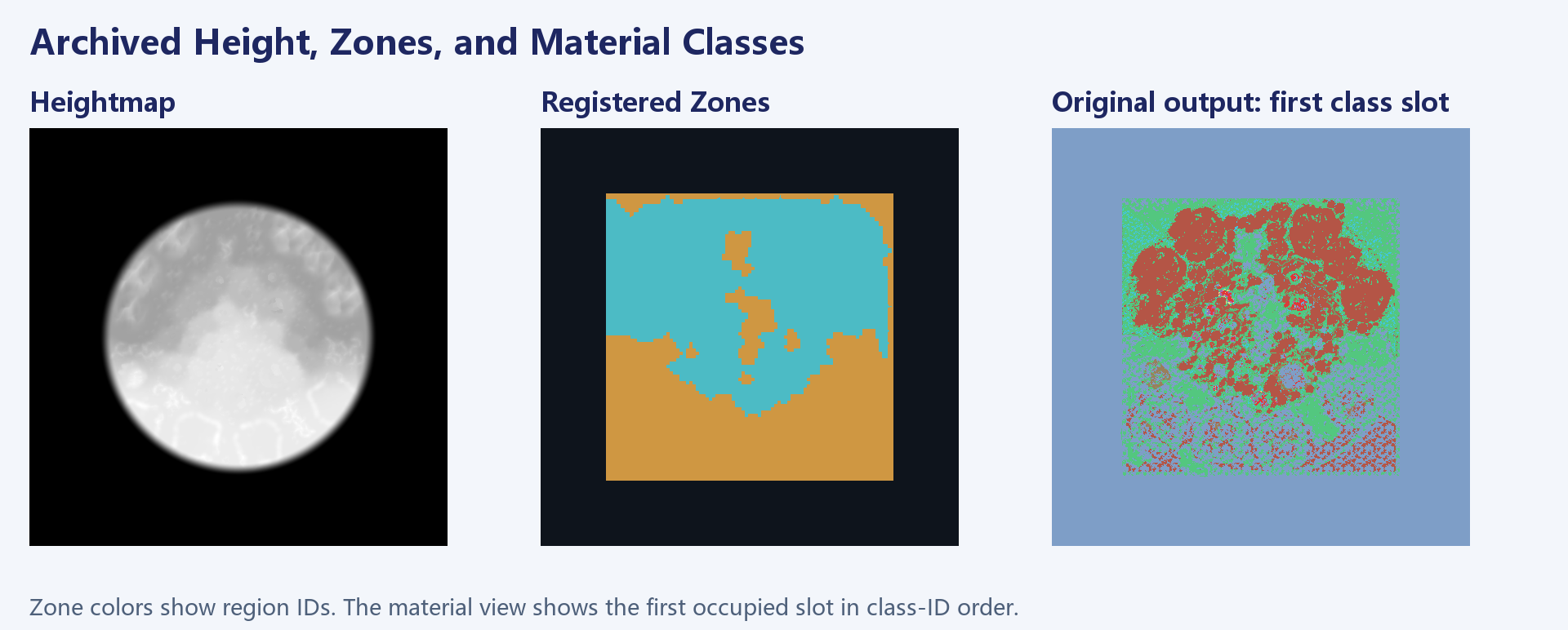
Zone Lookup and Material Draws
Zone lookup geometry writes generated_zones. The slope, noise, and route programs examined here use material Zone meshes and their vertex attributes. Their texture declarations contain no generated_zones input. Both paths share upstream information such as Cell adjacency and Zone labels.
The lookup map is useful for locating a region. To find where a material draw actually lands, examine its triangles and interpolated attributes, followed by the property height, noise, route distance, and destination channel. A region label can change abruptly at a boundary while material coverage remains continuous. A hard mask made from the labels would remove that transition.

Sand Classes 20 and 21
Classes 20 and 21 meet on the same slope, and both texture sets can be traced to their actual bindings. That makes them suitable for following the weights all the way to surface shading. Other classes are present in the close-up. Route and Raw draws can both contribute class 19, which provides a useful case for separating sources by their spatial distribution.
Class IDs route writes to channels and identify resources. The 32 candidate channels describe a working buffer, the three available class slots describe the output format, and the number of classes observed in a capture describes that sample. A texture array with the same layer count still needs its own binding and index mapping.
Zone Meshes and Raster Coverage
Material Parameters and Draw Geometry
The two neighboring Zones in the controlled replay specify base materials and separate slope, noise, and route draws. Both slope draws write sand class 20. Zone 48 favors shallow slopes, while Zone 49 favors steeper ones. Different thresholds, noise channels, and geometry can produce very different coverage from the same shader family.
A global rule such as material = slope > threshold ? rock : sand loses these Zone-specific responses. Keeping draw records by Zone lets each region apply its own slope range, noise, and coverage before writing to the shared class channel in sequence.
The controlled replay invokes the native mesh construction code on archived inputs to obtain vertices and indices. The recovered vertex declaration contains a float3 position, a UNORM8×4 attribute, and another float3 attribute. The stride is 28 bytes and indices are 16-bit. The original vertex shader must receive that declaration. Treating the packed attribute as four ordinary floats or dropping its fourth component changes the coverage seen by the shader. The native mesh replay uses archived request data with an explicitly chosen projection, target size, and resource inputs.
Coverage at Triangle Edges
The original vertex shader passes an attribute to the pixel stage. The slope, noise, and route programs read its v1.w component. The recovered meshes contain vertex values of 0 and 1, with intermediate values produced by interpolation. The weight calculation applies sqrt(abs(v1.w)). An interpolated value of 0.25 therefore contributes a factor of 0.5 before the remaining material conditions.
Rasterization establishes which fragments are covered. The pixel shader then combines the interpolated coverage with conditions such as slope and noise. A black texel in a weight image can mean that no triangle reached it, or that a covered fragment produced zero. Comparing the mesh mask and the draw’s weight output distinguishes the two.
An early test reused the Z mapping of a fullscreen triangle and clipped part of the recovered mesh. The remaining fragments still contained recognizable texture, but the extent of the draw had changed. The corrected test used an orthographic projection over the intended world bounds with a Z scale that kept the mesh inside the clip range. Holding the other inputs fixed then made the mesh and fullscreen cases comparable.
Mesh Coverage Compared with a Fullscreen Draw
A fullscreen test is useful for isolating a weight function. A flat input can be checked against the expected saturated result. A synthetic shallow slope can verify sampling of the designated noise channel and coverage attribute. At map boundaries, however, a fullscreen draw evaluates locations that the original geometry may never reach.
For the class 19 route draw in Zone 48, using the reconstructed native mesh reduced the number of positive candidate cells from 1,996 to 1,035. The overlap with positive cells in the final capture changed from 968 to 964. Most of the removed candidates were outside that overlap, so precision rose from about 48.5% to 93.1%. Recall remained near 41%. Other draws can supply class 19 in the final capture, and the reconstructed route distance also has its own input limits.
At a Zone boundary, overlaying the draw mesh on the registered lookup map shows where triangles cross the region labels. Clipping those triangles to the lookup labels can change the replay. A cross-section through the boundary can show where weights rise or fall. Holding the geometry, vertex interpolation, and shader inputs fixed is what lets the experiment attribute that change to a particular stage.
Slope, Noise, and Route Weights
Computing a Slope Weight from Neighboring Heights
The slope material reads the property-height resource generated_heightmap_properties_height. The original program establishes the declaration, sampling operations, and math. The property-height render target bound for the historical draw is absent from the archive. The archived heightmap supplies geographic context, while the test inputs make the controlled result reproducible. A height array of the same size is only a valid substitute if its resource role, scale, UVs, and sampler agree.
Let the property height be H(u,v). The original program derives the UV offset from mip and samples left, right, above, and below. This resembles a central difference, with the axis signs and scale taken from the original instructions.
size = 2048 >> int(mip + 0.5)
s = 1 / size
L = H(u - s, v)     R = H(u + s, v)
Vminus = H(u, v - s) Vplus = H(u, v + s)

n = ((size / 2048) × (L - R),
     (size / 2048) × (Vplus - Vminus),
     2)
q = 2 / length(n)

P(q) = ((-0.0187295 × q + 0.074261) × q - 0.212114) × q + 1.570729
angle = sqrt(1 - q) × P(q) × 0.636618
angleWeight = saturate((angle - angle_start) / (angle_end - angle_start))
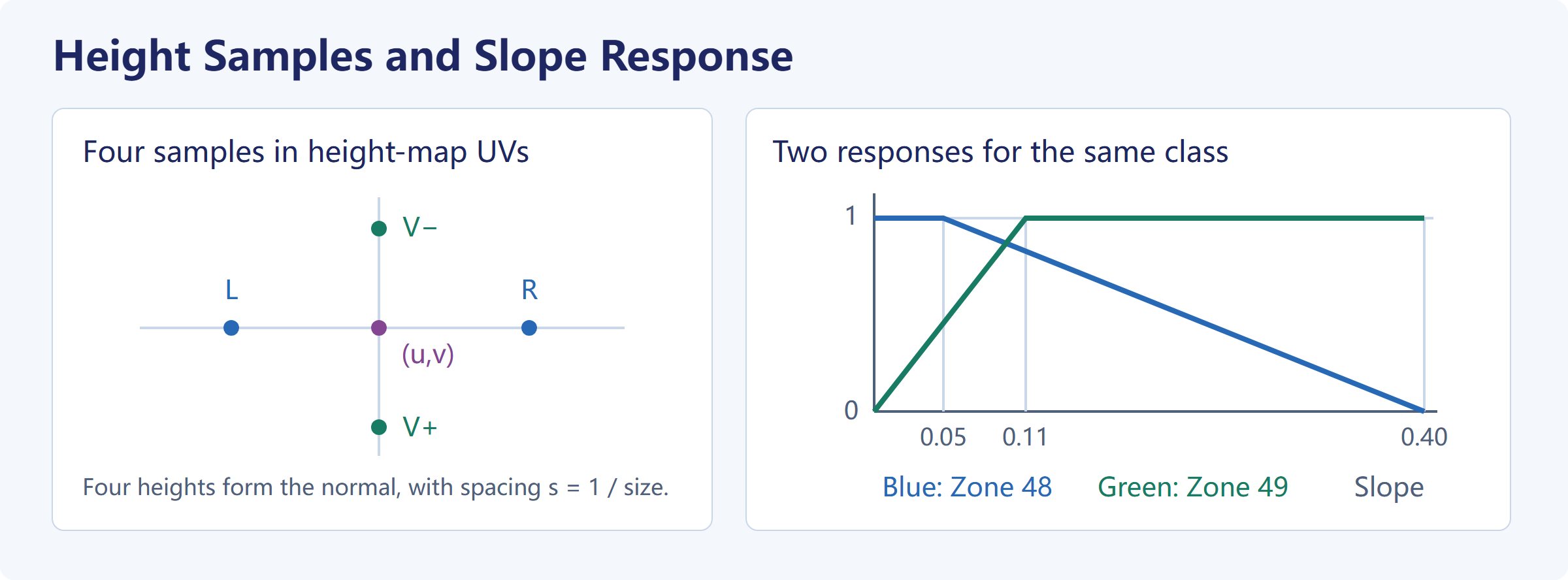
q is the cosine between the constructed normal and vertical. On a flat surface, n=(0,0,2) and q=1, so the angle term is zero. As the horizontal components increase, q decreases and the normalized slope angle rises. The polynomial and square root are the original shader’s approximation. An arccosine explains the shape of the response, while exact replay retains the original constants, operation order, sampling, and hardware precision. Both Zones use mip 0, giving s=1/2048.
The sign of the denominator determines the response direction. Zone 48 uses start=0.40, end=0.05, reaches its maximum at or below 0.05, and drops to zero at 0.40. Zone 49 uses start=0, end=0.11 and rises with slope. At a normalized slope of 0.08, the angle weights are about (0.08−0.40)/(0.05−0.40)=0.9143 and 0.08/0.11=0.7273, respectively. Mesh coverage and noise still have to be applied to obtain the amount written by the draw. Sorting the two thresholds would reverse Zone 48’s response.
Noise Modulation within the Slope Pass
The slope program samples a noise channel and combines it with vertex coverage and sharpness. Here N is the noise sample and saturate clamps to [0,1].
coveredSlope = angleWeight × noise_bias × sqrt(abs(v1.w))
dose = saturate(coveredSlope × (1 + noise_sharpness)
                + noise_sharpness × (N - 1))
| Zone | Destination class | angle_start → angle_end | noise_id / channel | bias | sharpness | noise_scale |
|---|---|---|---|---|---|---|
| 48 | 20 | 0.40 → 0.05 | 0 / R | 1 | 0.01 | 30 |
| 49 | 20 | 0 → 0.11 | 2 / B | 1 | 1 | 100 |
The instructions support interpolation between neighboring noise channels. These two settings are integers and select R and B. Scale applies to noise UVs generated by the vertex shader. Sharpness changes the numerical response in the pixel shader. Scaling the UVs changes the size or placement of the pattern. Increasing sharpness changes how much of that pattern reaches saturation or zero.
Using the same slope of 0.08, take an interpolated coverage of 0.25 and a noise sample of 0.4. In Zone 48, coveredSlope≈0.4571 and the dose is 0.4571×1.01−0.006≈0.4557. In Zone 49, coverage reduces the slope term to about 0.3636 and the dose is 0.3636×2−0.6≈0.1273. These are illustrative inputs. In the original GPU test, the flat control produced bytes 255 and 0 for the two Zones, the steep control reversed those values, and the shallow slope showed the noise modulation. Later writes determine the final material shares.
Separate Noise and Route Draws
The standalone noise materials also read noise and mesh coverage. In this case they write classes 1 and 3, respectively. Noise inside the slope program modulates class 20. Each operation has its own draw record and destination.
The route material reads a route-distance resource and combines it with noise and mesh coverage. The historical distance target was not retained. The replay feeds preserved route records through the original GPU distance program, then samples the resulting candidate on the chosen grid for the material draw. The distance field, the output of this one route draw, and the final class distribution therefore illustrate different steps. Other material inputs can account for additional class 19 regions.
A profile across a route edge shows changes in the same channel before and after the route draw. A profile from a slope into its neighboring Zone shows how coverage changes across the boundary. The dominant color in a final category map can conceal changes in the other retained classes. Dose and state images should share orientation, crop, and scale, with a separate close-up for narrow bands.
Weight Writes and Draw Order
Attenuating Old Weights and Adding a Class
The original program stores weights in RGBA8 render targets. Each draw first attenuates the existing values and then adds the new class. The verified fixed-function states are SRC=ZERO, DST=INV_SRC_COLOR followed by SRC=ONE, DST=ONE, with INV_SRC_ALPHA for the alpha channel in the first step. With uniform attenuation and a single destination class, the two writes can be expressed as follows.
oldAfterAttenuation[j] = Q8(old[j] × (1 - dose))
next[j] = Q8(oldAfterAttenuation[j] + paint[j])
paint[j] = dose if j is the routed category, otherwise 0
Q8 denotes the write to a normalized 8-bit target. Write masks, blend factors, and rounding at boundaries still follow the original shader and hardware. Two slope pixel programs supply the attenuation value and the routed class value. Class 20 goes to R in render target 5, using zero-based target indices. The eight RGBA targets give 32 channels. An RGB visualization of one class displays only one of them.
Suppose the starting point contains only A with a weight of 1. Drawing B with 0.6 gives ideal continuous values A=0.4, B=0.6. Drawing C with 0.5 then gives A=0.2, B=0.3, C=0.5. Reversing the two draws gives A=0.2, B=0.6, C=0.2. A keeps the same residual share, but whichever new class is drawn first is attenuated by the next draw.
Each 8-bit write can affect later steps. A residual of 0.49 byte units is lost on writeback. A floating-point implementation that rounds only at the end can carry that residual forward and occasionally change a close ranking between candidates. The hardware fixture ran the same producer inputs through the fixed-function states and matched the previously assembled eight targets byte for byte. Residual differences against the final game capture still leave property height, coverage, order, and later material inputs to check.

Intermediate Buffers in the Controlled Replay
The process images use one 512×512 grid throughout. The initial state assigns class 1 outside the two Zones, class 3 to Zone 48, and class 21 to Zone 49. The replay applies slope, noise, and route in Zone 48, then noise, slope, and route in Zone 49. These states are updated within the archived fixture’s region masks. The earlier native mesh experiments separately retained fragments across region boundaries to study geometry coverage. Each PNG visualizes one class byte, while the arrays preserve all 32 channels.
| Image | Meaning of a pixel | What it shows |
|---|---|---|
| Base class map | Initial class index in the fixture | The material each Zone starts with |
| Draw dose | Output of one weight producer | Where that draw contributes |
| Accumulated weight | Current class value in the target | The result after all preceding draws |
| Step difference | Current value minus previous value | Where the class increased, decreased, or stayed constant |
| Merged weight | Class share decoded from the packed word | Whether the class survived selection and its retained share |
The Zone 48 noise draw writes class 1, but it can also darken the accumulated class 20 image. The attenuation step reduces the old values before the second write adds to class 1. Class 21 can also lose weight during a draw that writes a different class. The before and after buffers, together with the destination class, identify why a region darkened.
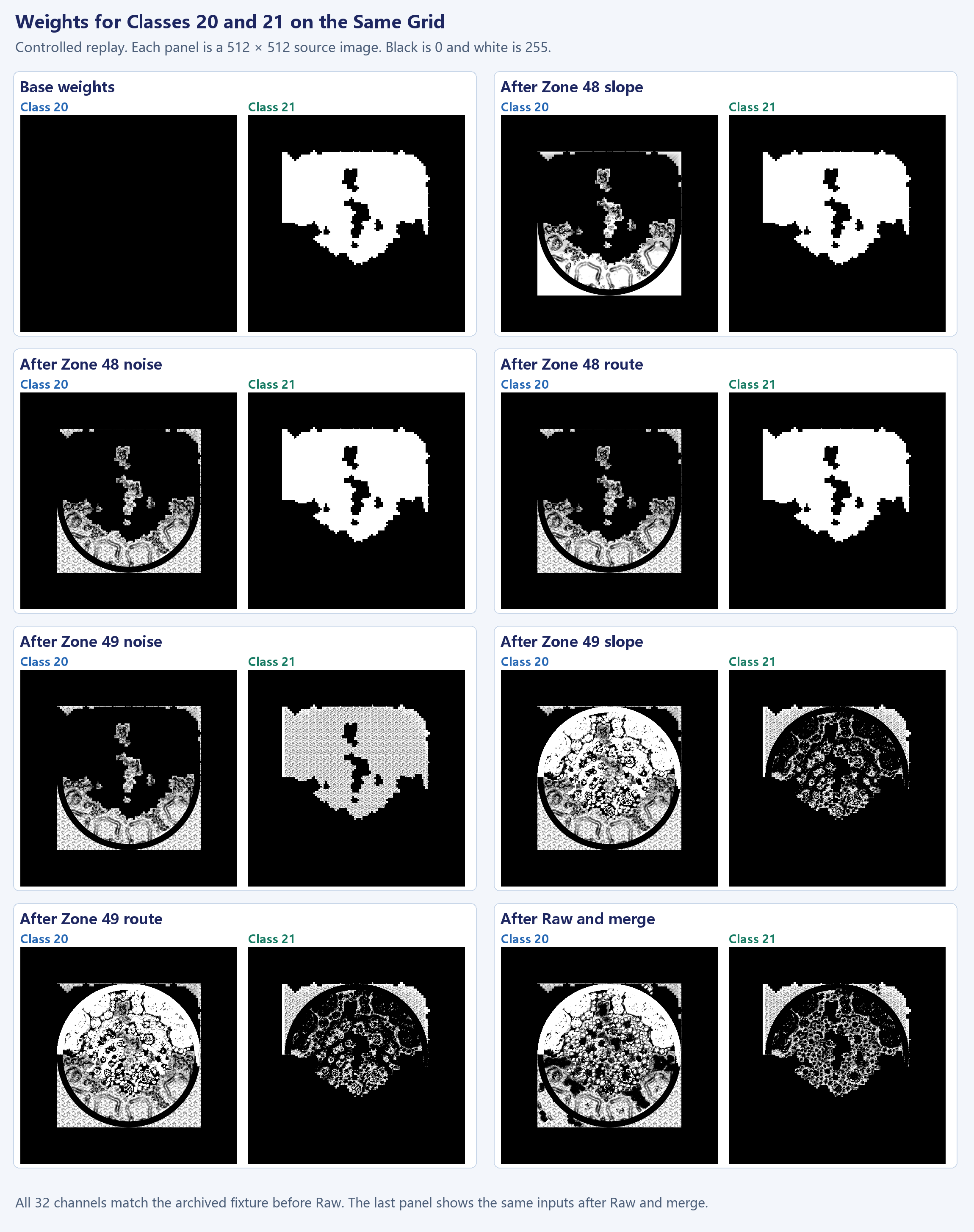
Raw draws use source material images and instance transforms to write local patterns. Overlay draws have their own inputs and coverage. A later class 19 draw can widen an existing route band, while a draw to another class can attenuate it. Class 19 can also remain positive in the pre-merge buffer but disappear from the final map when other classes outrank it. The full channel array distinguishes these cases.
Tracking the Weights at One Sample Cell
Cell (217,124) in the 512² grid is registered to point P later in the article. The first three draws are in Zone 48 and leave this cell unchanged under the fixture’s region mask. The Zone 49 noise draw gives class 3 a value of 162 and leaves class 21 at 93. The slope draw writes class 20 and attenuates both existing classes.
| Step | Class 3 | Class 20 | Class 21 |
|---|---|---|---|
| Base and end of Zone 48 | 0 | 0 | 255 |
| After Zone 49 noise | 162 | 0 | 93 |
| After Zone 49 slope | 45 | 184 | 26 |
| After Zone 49 route | 45 | 184 | 26 |
| After Raw, before merge | 0 | 185 | 70 |
With a dose of 184, the attenuation factor is (255−184)/255. The old values 162 and 93 become about 45.11 and 25.89, then round to 45 and 26 on writeback. The route draw does not change this cell. After Raw drawing, class 3 has already reached zero, and classes 20 and 21 are 185 and 70. The loss of class 3 therefore precedes the merge shader’s selection.
To repeat the check at another location, inspect W[y,x,:] at each step. Convert the bytes to a signed type before subtraction, since 10−20 wraps to 246 in an unsigned byte. The process maps share the same 0–255 scale. Small changes along a route can be shown separately in a difference image with its display gain identified.
The original material construction code provides the order of entries in each Zone array and the integer keys sent downstream. The command handler writes the key into a resource field that a general draw path can use when sorting. That establishes a code path for sorting. The historical active queue still requires a draw record. The illustrated fixture initializes the base once, then draws the materials in array order without clearing the target between Zones. The archived Raw fixture follows those writes.
The eight RGBA8 targets before Raw contain 512×512×32 = 8,388,608 channel bytes. The per-class PNGs are only views of that data. Files named premerge_target in the package are a later checkpoint, after Raw has run and before the merge. Compare each array to the checkpoint it represents. A difference in the full word can then be split into class selection and weight-byte differences.
Route and Raw Sources for Class 19
Both route and Raw draws can leave the same class ID. Route distance produces narrow bands, while projecting a Raw source through an instance transform can leave more irregular patches. The analysis registered three datasets on the same grid: positive class 19 values in the final capture, positive route candidates, and world-space projections of class 19 source texels from Raw materials.
Zone 48 had 2,352 positive class 19 cells in the capture. Of these, 968 overlapped the route candidate. Of the remaining 1,384, 1,163 overlapped the Raw projection and 402 matched its complete material word. In Zone 49, 1,692 of 1,694 positive cells overlapped the route candidate. The two regions show a route-dominated distribution and one with additional localized Raw input.
Shifting the Zone 48 Raw projection as a negative control sharply reduced the matching count outside the route. Matching words concentrated at the registered position are stronger evidence than isolated matches in repeating textures. Some points still lack a direct match. Nearby projections can be affected by filtering, coverage, or registration. The late archive only records program associations for part of the instance set, so the spatial match constrains the likely source while the historical draw activity remains limited to what was recorded.
Expanding the route threshold could increase overlap while creating spurious bands. It would still leave the correspondence between source textures and local Raw patches unexplained. Unmatched points remain useful for checking the distance candidate, filtering, and registration separately.
Class Selection and 32-Bit Packing
Candidate Channels and Output Slots
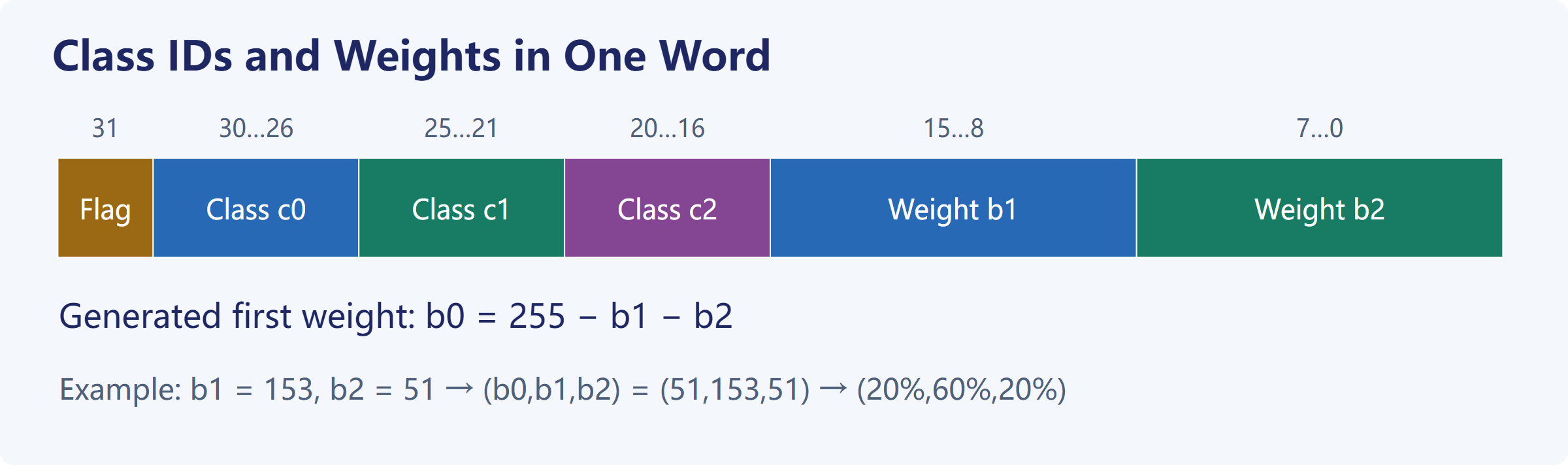
The 32 working channels let draws write to independent destinations and attenuate prior values. Subsequent material passes usually need only a few candidates at each location. The original merge shader selects up to three classes and packs their IDs and weights into a single 32-bit word.
On a tightly packed 4096×4096 grid, 32 bytes per texel take 512 MiB, while 4 bytes take 64 MiB. Actual VRAM usage also depends on the resource lifetimes, allocation, and other targets in flight. The downstream reader can recover the selected IDs and explicit weights from one word.
The pixel shader reads eight RGBA targets and uses a comparison network to retain up to three classes with the highest weights. It then orders the occupied slots by class ID and encodes the normalized second and third weights as bytes. The instructions zero weights below 0.001. In the R8 control, channel 0 drives the high-bit flag and sets it when the channel is saturated. In the measured generated word at P, the trailing class 0 is an empty slot with zero weight.
An original GPU test used classes 1, 3, 20, and 21 with channel values of 10, 20, 200, and 25. The merge kept 3, 20, and 21, totaling 245. Normalization and conversion produced 208 and 26 for the second and third slots. Decoding the remainder gives 21 for the first. The original floating-point division and conversion determine the low bytes. Integer ratios explain this example but may differ by a code value at a boundary.
The comparison network is sensitive to the other candidates when classes tie at the cutoff. In one control, classes 19 and 21 tied for third. With classes 28 and 29 ahead of them, the GPU retained class 19. With classes 20 and 3 ahead, it retained class 21. Exact replay requires the comparison network. The ascending order of occupied slots only applies after selection.
Let c0,c1,c2 denote the three class slots and b1,b2 the explicit weight bytes. Decode the raw bits before filtering.
flag = (word >> 31) & 1
c0   = (word >> 26) & 31
c1   = (word >> 21) & 31
c2   = (word >> 16) & 31
b1   = (word >>  8) & 255
b2   =  word        & 255

generatedWeight = (255 - b1 - b2, b1, b2) / 255
The remainder formula decodes the generated material map. The runtime material shader reads the two low bytes of imp_map as the opacities of their respective slots. The first runtime slot follows a separate rule.
For a pixel containing classes 3, 20, and 21 with explicit bytes 102 and 51, the first weight is 255−102−51=102. The generated shares are 40%, 40%, and 20%. With the same class order and bytes of 153 and 51, class 3 has 20% and class 20 has 60%. A map of the first slot shows the encoding order. To show the dominant material, select the valid class with the highest weight.
Class 31 has a sentinel role. A field in the word can exist without a corresponding material draw. The decoder must respect the downstream rules for valid classes and empty slots. A low weight byte can change even if its third class is still a sentinel. A word-level difference can reveal a change in encoding or shader behavior. A visible change also depends on class filtering, bindings, and blending.
Flag Bit and Discrete Classes
The original variants consume the high bit at different stages. The non-tessellated path can discard in the pixel shader. The tessellated path can zero the tessellation factors in the hull shader. The archived generated map contains texels with the bit set. Counting discarded raster fragments would additionally require the active variant, the resource it read, and the actual draw inputs.
Class IDs are discrete. Interpolating halfway between IDs 3 and 21 would yield 12, a material absent from both samples. Filtering the packed word as color can also let arithmetic carries cross fields. Decode each neighboring word, then accumulate or select within matching classes. One original imp_canvas path does this with four neighboring texels.
For an illustrative four-neighbor sample, suppose both left texels contain only class 20. The upper right texel contains classes 20 and 21 in equal proportions, and the lower right contains classes 21 and 19 in equal proportions. With four equal spatial coefficients of 0.25, the totals are 0.625 for class 20, 0.25 for class 21, and 0.125 for class 19. The real shader also processes variant inputs, displacement data, and candidate pruning. The example isolates the reason for decoding before interpolation.
Checking the Original Merge Output
The archived 4096² map contains 16,777,216 texels and roughly 400,000 distinct output words. The test built candidate channel inputs from every distinct word and ran them through the original DXBC merge shader. Most matched immediately. Some required a small search over the three candidate weights. Every distinct word could be produced in the isolated GPU replay, including unusual classes and flag combinations.
The merge is many-to-one. Two inputs can retain identical classes and encode the same word despite differences in the discarded channels. Quantization can also erase differences. Inputs inferred from output words are useful test vectors for the merge. Recovering the historical targets after Raw and Overlay would require those targets’ readbacks or an independently verified forward reconstruction.
The forward test starts with draw inputs and compares the resulting words. In one high-resolution control, five Raw inputs replayed with original GPU programs were placed back into an existing draw sequence, leaving the other inputs unchanged. The original merge shader matched 15,187,763 of 16,777,216 words, about 90.53%. An independent 512² control matched 261,774 of 262,144 registered cells. The two tests used different candidate inputs, resolutions, and boundary sampling.
Runtime Class Filtering and Material Blending
Generated and Runtime Material Maps
The archive identifies generated_materials and imp_map as separate resources. The generated output was saved at 4096². At runtime, imp_map is configured as a two-channel unsigned integer target. The imp_canvas pixel shaders examined here write X, and the imp material shaders read the packed word from X. The field layout is shared. Each stage has its own writer, resource, and interpretation of the values.
One runtime path reads neighboring material words in the pixel shader. The other obtains candidates earlier in the geometry pipeline and passes classes and weights to the pixel stage. Both can output the same layout, with different sampling and coverage rules.
Similar dimensions and formats can be used to build a controlled input. The available named-resource records leave open whether the historical draw bound the captured generated_materials as material_map. That requires the actual view, constants, SRV, and draw queue.
Non-Tessellated and Tessellated Paths
In the non-tessellated path, the VS supplies coordinates and the PS reads four neighboring words from material_map. A class may appear in more than one corner and must be combined before further processing. This variant discards in the pixel shader. In the tessellated path, class data enters during vertex processing. The high bit can cause the HS to set all six tessellation factors to zero. For an accepted patch, the DS evaluates the surface position from geometry and array data. The PS receives constant-interpolated class IDs and linearly interpolated weights. The VS reads material_map in this variant.
The two variants have different debugging entry points. A PS discard occurs after raster coverage has been established. Zeroing tessellation factors changes earlier geometry work. For a hole or silhouette, inspect patch inputs, factors, and DS positions in the tessellated path, or the four lookups and discard condition in the non-tessellated path. The final color buffer alone cannot locate the first loss of coverage.
The Sandy variants examined here declare 224 bytes of object constants in the VS, PS, and DS where present. The HS does not declare this buffer. The ordinary Raw VS uses a separate 144-byte layout. The size can help identify a candidate, but the field use and program must agree. Reusing an object buffer across unrelated stages can leave plausible matrices alongside scales and UVs from the wrong object. Capturing bindings, coverage, and output per stage makes these errors traceable.
Displacement Array Use in PS and DS
Both verified imp_canvas pixel programs read the 32-layer terrain_displacement_map array. The instructions subtract one from a valid class ID to obtain the layer and handle sentinel class 31. The resource swizzle and register write masks show that these samples read X. The tessellation DS separately reads XY during position evaluation.
The non-tessellated ablation held geometry, constants, and coverage fixed and changed only the array. Setting X to zero changed the weight fields of 6,942 packed words out of 30,800 covered pixels. Setting Y to 255 left the output words unchanged. This establishes a weight dependency on X in that pixel program. The effect of Y on geometry belongs to a separate DS position test.
The 27-layer BC5 resource retained in a late frame is separate from the 32-layer RGBA8 runtime array. Its channels can be spatially associated with R and G of the Sandy displacement source. The source image also contains B and A, which feed the color path and cannot be supplied by the two-channel array. The shader declaration and actual binding establish which array a stage uses.
Opacity and Ordered Compositing
The generated map encodes three normalized shares with two explicit bytes. The verified runtime consumer treats the two low bytes as slot opacities, and the first slot starts at 1 in the reproduced path. Each material PS matches the slot IDs against its material_index and accumulates the matching values. The original instructions discard the fragment below 0.001, or write the sum to the color target’s alpha. The verified blend state uses SRC_ALPHA / INV_SRC_ALPHA.
C_next = C_source × alpha + C_old × (1 - alpha)
Assume the first layer covers the pixel and each of the three distinct classes draws once, with opacities (1,a,b). After drawing C0 and C1, the color is (1−a)C0+aC1. Drawing C2 attenuates both earlier terms.
C_final = (1 - a) × (1 - b) × C0
        + a × (1 - b) × C1
        + b × C2
For a=0.25,b=0.50, the effective coefficients are (0.375,0.125,0.50). The generated-map remainder formula would give (0.25,0.25,0.50). The third draw covers part of the second layer, reducing its contribution from 0.25 to 0.125. Both vectors sum to 1, so checking the sum cannot distinguish them.

The order of IDs in the word is an encoding convention. The static FRONT_BACK setting concerns the draw queue. Changing the order of material draws can change the resulting color. The historical result also depends on sort keys, depth and stencil, the initial target, and variant bindings. The current Blender blend uses a declared order and corresponding coefficients. A control that exchanges the draw order measures sensitivity under that control’s inputs.
Reading Both Maps at the Same World Position
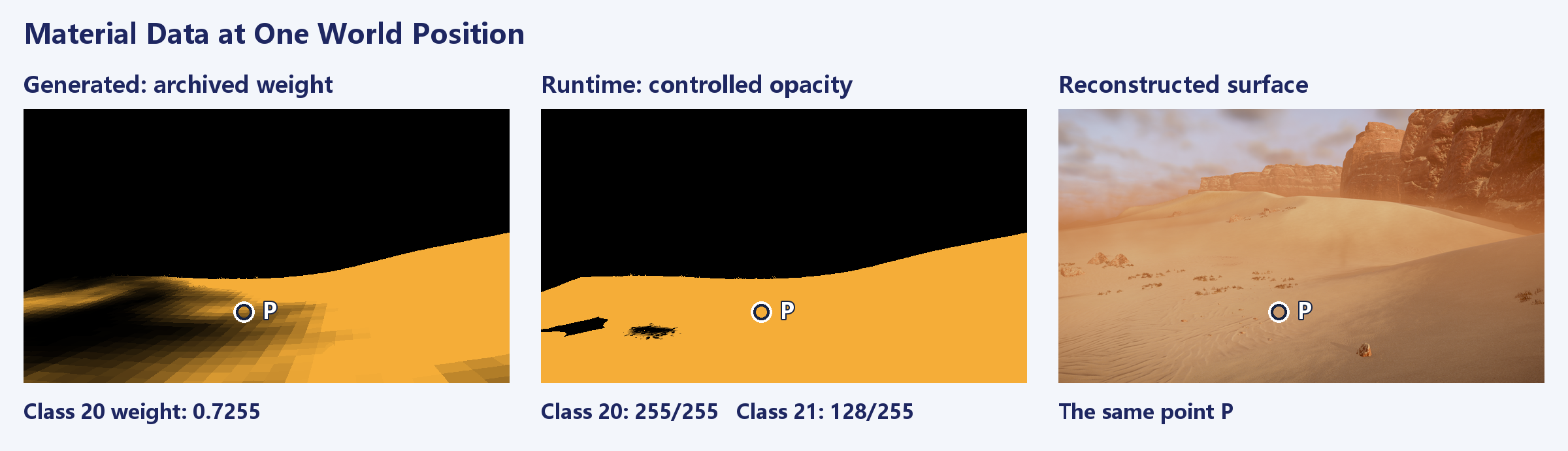
Blender’s Position AOV maps point P to approximately (−153.568,526.883) m. The archived generated map covers [−1024,1024] on a 4096 grid. The runtime orthographic map has its own world bounds (x0,y0,x1,y1). Both views use nearest-neighbor lookups, with texture Y reversed relative to world Y.
u_gen = floor((x + 1024) × 2)
v_gen = floor((1024 - y) × 2)

u_run = floor((x - x0) / (x1 - x0) × 4096)
v_run = floor((y1 - y) / (y1 - y0) × 4096)
| Data | Sample coordinates | Material word | Classes and values |
|---|---|---|---|
| Archived generated map | (1740,994) | 0x52A04600 | Classes 20, 21, and 0. The generated shares are 185/255 for class 20, 70/255 for class 21, and zero for the last slot |
| Controlled runtime orthographic map | (574,2872) | 0x0295FF80 | Slots 0, 20, and 21. Classes 20 and 21 read 255/255 and 128/255 from the explicit bytes |
At P, class 20 occupies the second runtime slot. Its opacity of 1 comes from the explicit byte 255. The reconstruction draws class 20 first, then covers about half of it with class 21. The middle image shows class 20 opacity and is nearly uniform across much of the surface. The visible ripple transition still varies with class 21 coverage and both texture sets.
The earlier 512² sample also produced 0x52A04600, matching the complete word at the registered capture point. Other positions, especially narrow route bands and material boundaries, need their own comparisons. The three panels are aligned in world space, but the runtime map has a different sampling footprint. The difference 1−185/255 crosses both a change in representation and a change in execution conditions.
Sand Textures and Surface Shading
Original Textures and Sample Bindings
Classes 20 and 21 have similar base colors. Their close-range differences are easier to see in displacement and normals. After saving and reopening the Blender scene, the near and macro branches for each class were checked against their original albedo, displacement, and NAR textures and mip data.
Part of class 21’s UV mapping is reconstructed. The same source texture can produce a different pattern density, orientation, and frequency when its sample positions or scale change. Reproducing a historical draw would require the UVs, gradients, LOD, sampler, variant, and blend coefficients in addition to the texture bytes. Texture identity and reconstructed sampling are tracked separately.

A Source Texture Shared by Displacement, Weights, and Color
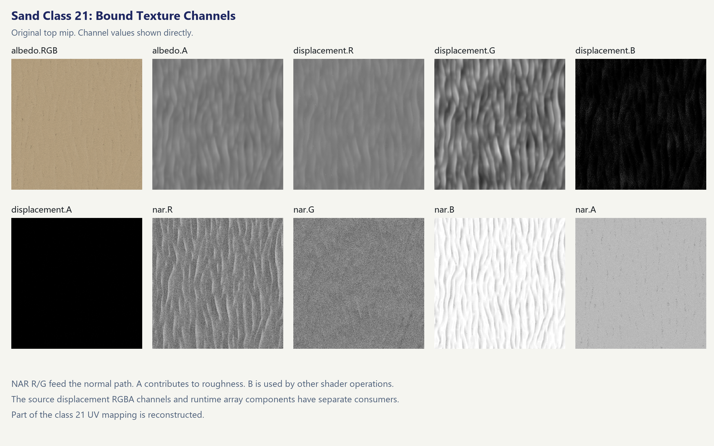
The original RGBA displacement texture feeds several paths. The array derived for later stages has different consumers for its components. Source R and G can contribute to displacement or to the inputs from which it is derived. Source B and A also appear in the original material’s color grading. A grayscale export would omit the data needed by those other paths.
In the verified imp pixel programs, the color grading path transforms the input color C in a main, secondary, and masked group. It then interpolates using B and A from the displacement texture.
Cmain   = saturate(Mmain(C))
Csecond = saturate(Msecondary(C))
Cmasked = saturate(Mmasked(C))

Cgraded = lerp(lerp(Cmain, Csecond, B), Cmasked, A)
The expanded coefficients are (1−B)(1−A), B(1−A), and A. With A at 1, the masked result covers both earlier terms. With A at 0, B alone sets the transition between the main and secondary groups. For B=0.25,A=0.10, the coefficients are 0.675, 0.225, and 0.10. Treating A and B as independent shares with (1−B−A)Cmain+BCsecond+ACmasked shifts each of the first two coefficients by 0.025. The resulting error follows the texture’s A boundaries.
Dual-sample variants read the relevant components at two UVs and combine them with an interpolation value derived from albedo alpha and the material’s sharpening setting. Albedo alpha affects sampling or modulation within one material. The alpha written to the render target comes from the runtime map and determines how this draw covers the previous color.

NAR Normals and Surface Response
The NAR R and G channels are mapped to signed values for the local normal. For a unit vector on a hemisphere, the reconstructed components x,y give the geometric relation z=sqrt(max(0,1−x²−y²)). The original consumer determines the axis assignment and signs. The terrain tangent basis then transforms the direction to the shading space. Whether a ripple changes the actual silhouette still depends on geometry displacement. Comparing normal and position outputs separates the two effects.
NAR A enters the confirmed roughness-related path, which includes 0.045+0.955×saturate(A). The material and lighting determine how that value appears in the final image. B participates in glint or related shading calculations. The channel sheets preserve the values as stored. Their meaning comes from the original instructions rather than an ORM naming convention.
Both sand albedos have similar colors. The displacement pattern and changes in local normals explain why switching classes can produce a pronounced ripple response under light, even when the base colors remain close. A grazing light angle can make those directional differences easier to see. The following comparison uses the same lighting for all three variants.
Same-Camera Material Comparison
The three close-ups share the same Blender camera, crop, geometry, World, Sun, exposure, and sampling. The left image uses the surface properties of class 20 alone, the middle uses class 21 alone, and the right uses the current blend. All three disable the cached lighting, fog, and post-processing tied to the fixed main view. Their linear HDR buffers are displayed with the same gain, Reinhard mapping, and sRGB encoding.

The comparison varies surface color, normals, and roughness while retaining the geometry. Class 21 has more continuous lateral ripples, which weaken in parts of the mixed surface without a corresponding change in the terrain outline. Measuring the vertex-height change due to one class requires a position or depth comparison under matched geometry inputs. The displacement control below addresses that question separately.
Carrying GPU Weights into Blender
From Screen Coordinates to World Coordinates
A weight buffer projected from a single view can reproduce the distribution for that camera. Moving the camera changes the footprint and visible area. The reconstruction instead generates a world-space atlas from the controlled original GPU output. It retains the original producer PS and displacement stage and uses the near-field mesh’s XY bounds to define an orthographic target about 67 m across. Blender samples it by world position.
The atlas supplies per-class opacity, effective coefficients for the declared blend order, coverage, and pair validity. A world point (x,y) maps to normalized atlas coordinates before a lookup. Some classes are zero across the patch, so the graph need only evaluate the complete texture path for relevant classes. Comparing packed fields and floating-point exports on write, then checking the Blender node inputs on read, separates data-transfer errors from shader errors.
Projection changes the derivatives and LOD. When the 4096 orthographic atlas was reprojected onto the reference view, the dominant class agreed at about 99.82% of the selected interior pixels. At some sharp edges, the maximum absolute opacity error still reached 1. Cross-checks against two other original GPU views also found such extremes. The atlas provides a stable reconstruction input across this patch, with occasional class changes near boundaries.
A switch from class 20 to 21 can be visible even when most opacity differences are small. Marking pixels whose dominant class changes shows how they align with material boundaries. Percentiles help characterize the interior. Normals, roughness, and glint can then be inspected separately where needed.
Scalar Weight Outputs in Cycles
An earlier Blender graph exposed several groups of vector outputs at once and hit a stack limit in the Cycles shader virtual machine. The rendered material coverage dropped sharply even though individual image nodes returned valid values in local probes. The revised graph sends the scalar coefficients, opacities, and coverage directly to their consumers. It avoids retaining temporary vectors just to extract one component. The numerical method stayed the same, and the full scene passed the coverage check again.
When local probes are correct but large areas disappear in the render, check Cycles compilation and actual coverage first. Once the graph evaluates, inspect the class coefficients and source bindings for crossed connections between surface layers.
Reopening the Saved Scene
After reopening the scene, the near and macro branches for classes 20 and 21 still point to their respective original textures. The final render checks are described below.
The finished scene uses the full display path. The earlier material triptych disables fixed-view caches to isolate the surface properties under the same lighting.
From Material Outputs to the Final Image
Sand Displacement and Surface Highlights
The blend determines which textures contribute at each location. The tessellation domain shader reads X and Y from the displacement array, computes a transition and displacement amount, then applies the scale to vertex height. The surface shader reconstructs local normals from NAR and computes roughness and glint. The former can move the surface and affect its shadows. The latter changes the response to light. The earlier material triptych held geometry fixed, so the displacement comparison uses a separate control.
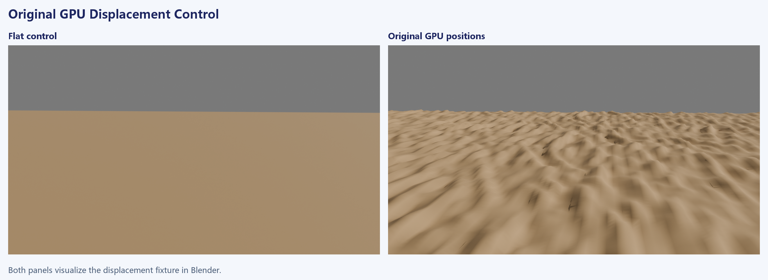
The displacement path maps each selected class to an array layer, then computes sample coordinates according to the variant. Original code can read UV mapping and flow data, and some branches generate two rotated coordinates. A single repeating grayscale map can create relief but loses these scale and transition rules. The controlled test first checks the positions produced by the original program and then uses those positions in Blender. The final main view uses reconstructed settings. The displacement scale bound for the historical draw remains unverified.
Original sand materials 19, 20, and 21 use glint_intensity=0.5 and glint_amount=0.2. The retained material properties agree with the authored assets, and the original pixel programs read the corresponding fields. In an earlier same-camera test, wiring in the recovered color and normal path changed the foreground’s light response while leaving the long ripple pattern recognizable. The final build checks the original GPU path under the current view and inputs, with part of class 21’s UV mapping still reconstructed.

Replacing Lighting Contributions from the Same Render
Blender’s Combined pass already includes World and Sun contributions. Adding original GPU lighting directly would count both twice. The final scene obtains Combined, World, and Sun from the same render layer, subtracts the latter two, and adds original GPU lighting replayed with the current scene inputs.
L_surface = Combined - World_live - Sun_live + L_original
L_original includes environment lighting, subsurface scattering, and shadowed sunlight under the reconstructed inputs. Because World and Sun come from the same render as Combined, the subtraction uses the same coverage, material, and camera sampling. Mesh emission remains in the residual. The source meshes in the frozen scene were checked to have zero emission. Lighting and composite caches need to be rebuilt when the camera, scene, or render settings change.
Atmosphere, Dust, and Display
Surface lighting first passes through the atmosphere composite. Depth and coverage select the terrain or sky path, and atmosphere and cloud outputs contribute here. Aerial perspective reduces contrast on distant cliffs while the surface lighting retains the foreground ripples. The composite then adds dust and particles in sequence, using premultiplied color.
L_dust = L_atmosphere × (1 - a_dust) + C_dust_premultiplied
L_hdr  = L_dust × (1 - a_particles) + C_particles_premultiplied
The HDR composite proceeds to temporal accumulation, exposure, and display conversion. The fixed-view reference uses eight jitter phases, with the inputs retained for each phase and the original post-processing executed on them. The first three panels below are buffers from the same phase, shown with a common HDR display transform. The fourth is the delivered Blender image after the eight-phase process.

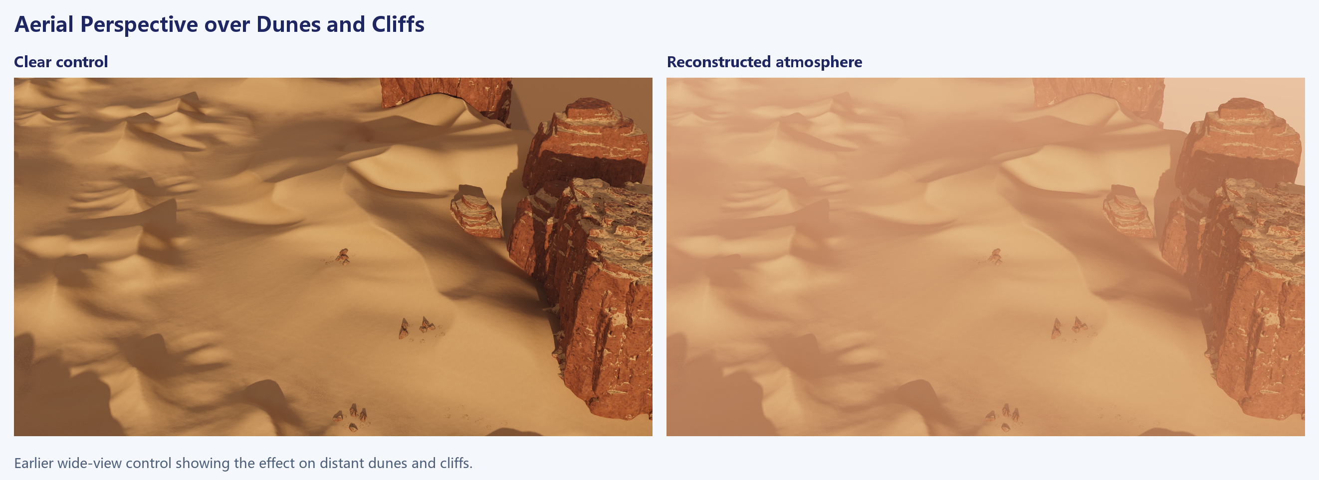
The earlier wide view makes the atmospheric effect easier to see. The clear control retains the dark shadows from the right-hand cliffs and the unlit sides of distant slopes. After the atmosphere is applied, contrast falls across the slopes, depressions, and cliffs without moving the dune boundaries. The buffers above show the final main view’s compositing steps.

The final check compares renders from the reopened Blender scene with the corresponding reconstructed original-GPU reference. The largest per-channel difference was 4 on a 0–255 scale. The two independent renders were identical. The wide view and early glint comparison illustrate individual changes. The current stage-by-stage verification applies to the fixed main camera.
Locating Differences in the Pipeline
Shifted Material Boundaries
Check map registration first. Align the extents of the height, Zone, and material maps. Verify the image Y direction and whether coordinates refer to texel centers or edges. When reducing a 4096² map to a 512² grid, retain the exact sampling coordinates. Averaging can soften narrow route bands and eliminate some positive weights. Nearest-neighbor sampling preserves the chosen values but can miss features between sample points.
Once the maps align, use the shape of the residual to locate the stage. An error along a Zone outline points to mesh coverage, projection, or interpolation. A change inside the outline that follows the terrain slope points to property height, mip, or the slope thresholds. A narrow band calls for checking route distance, covered fragments, and later contributions to the same class from Raw. If placement is correct and the weights are low across a region, check the noise channel, sharpness, R8 attenuation, and order.
Packed Words and Channel Errors
Compare all 32 candidate channels before judging a difference by eye. One or two codes can swap candidates near the cutoff. A change in the selected IDs can then shift multiple fields because the occupied slots are sorted. If only weight fields differ, inspect quantization and draw inputs. If class fields differ, inspect the ranking and sentinel handling. If the high bit differs, inspect its input channel and the stage that consumes it.
The same packed word can also conceal differences outside the top three. Recovering the draw process requires comparing the render targets before the merge. Implementing the consumer requires a correct decode and the right interpretation for that stage. The original GPU merge test checks representability of the output. The before-Raw checkpoint checks all 32 channels for its particular set of controlled inputs.
Material Bindings and Display Differences
Confirm the texture identity and UVs in the single-class views. If classes 20 and 21 already look alike in isolation, inspect the bindings, UVs, and normal reconstruction. If the individual surfaces look right and the mixed region differs, inspect opacity decoded from imp_map, matching-class accumulation, draw order, and discard. If the problem only appears with the fixed-view caches enabled, check lighting, shadows, fog, and post-processing.
Use the same camera for both material controls and the full display path. A defect at the same material boundary in both views warrants tracing the classes and weights. A defect present only in the full display points to the view-dependent inputs.
Class, Weight, and Pixel Differences
At a class 20 sample, a one-byte discrepancy can be measured in the pre-merge channels or decoded weights if the selected classes agree. If two candidates exchange the last retained slot, record it as a selection difference. If the generated words agree but ripple direction differs, the material sampling needs its own check.
Subtracting whole words gives a poor visual metric. A bit change in a class field produces a large integer difference even if the two materials look similar. Identical words can still produce different surfaces when the UVs or mip levels change. Record class sets, decoded weights, displacement, and visible pixels separately at registered world positions. Averages describe the common case. Keeping coordinates for boundary and outlier samples makes it possible to trace the first change in a draw or binding.
Reconstruction Scope and Remaining Inputs
The controlled replay matches the archived weights before Raw byte for byte. The saved Blender scene preserves the verified texture bindings for sand classes 20 and 21.
A full reproduction of the historical request would still require the actual draw queue and bindings, the property-height resource, and the original targets before merging. The Blender reconstruction uses a world-space orthographic atlas for local weights. Part of class 21’s UV mapping and view-dependent lighting, fog, and post-processing use reconstructed settings. A different camera or weather condition requires checks against the corresponding sampling and lighting inputs.