
The image below compares the reconstructed terrain on the left with the height reference for the same request on the right. This article follows the generation pipeline to explain how mountains, local relief, and location shapes are produced.

Figure 1: A comparison in the Web 3D viewer. Both sides use the same canvas, camera, lighting, and color scale, with 1:1 vertical scale and a display disk of radius 625 m. The left side shows the generated result after natural Stamp and location texture drawing; the right side is the final height reference for the same request.
The oblique view helps compare mountain silhouettes, slope continuity, and local relief. Camera, lighting, and vertical scale are identical; pixel errors are measured separately from the original height data. The 625 m disk defines only the display area. It does not establish validation of the entire 620–680 m outer blend band. Exact code agreement and error across the complete square heightmap are examined at the end.
This article follows From Configuration to Reverse Engineering: Terrain Reconstruction, a Web Prototype, and C++ Migration. That article used configuration relationships and reference samples to constrain repeatable reconstruction, retaining proxy algorithms where calculation rules or assets were missing. The earlier multiplayer article, From Playable World to Multiplayer Session: UE5 Runtime Terrain, POI Placement, and Dedicated Server Synchronization, discussed runtime integration and synchronization. Here, the focus is the generation of the height data used at runtime.
This article independently rebuilds the heightmap for a fixed tundra request using the original algorithm’s pipeline. For the fixed tundra request examined here, the implementation follows confirmed original configuration relationships, resources, and calculation rules. It computes source heights, corner weights, rasterization, smoothing, location support, and local height composition in their actual stage order. These rules and inputs drive generation. Reference heights validate stage results and final pixel errors rather than serving as the input base surface. Natural Stamp and location shapes come from their respective static height assets.
The following sections describe each stage’s inputs, rules, and outputs. Validation covers the height pipeline for this request; other biomes, uncovered branches, and the complete scene runtime require separate verification.
A procedural map must accommodate continuous mountains, gently sloping ground, local ridges, and mission locations. Mountains need large-scale spatial organization, local features need distinct shapes, and ground around locations must join the surrounding terrain. Different stages address these requirements, ultimately producing a heightmap that rendering, collision, and placement systems can query.
This article traces a tundra generation pipeline from configuration to final height pixels: organize regions and height relationships, generate a continuous base surface, calculate location support, draw natural Stamp and location height textures, blend the outer area, and encode floating-point heights as R16. Complete location layout and scene scattering are reserved for later articles. This installment follows one fixed request from input to final R16 data.

Figure 2: Follow the arrows to read the stage relationships. Steps ①, ②, and ⑧ are mechanism diagrams; ③ shows the actual planar location layout. Steps ④–⑦ show actual height results for the same central area. Outer blending and encoding are detailed later.
Read Figure 2 from ① to ④ across the top row, down to ⑤, then left along the bottom row to ⑧. The pipeline prepares configuration and spatial inputs, modifies the height field, and delivers the result to scene systems.
Step ①, Request and Configuration, establishes candidates and parameters. The seed and scene conditions participate in selection; recipe index 19 identifies the configuration, while execution draws random values and advances the random state. Step ②, Regional Structure, associates configuration with boundaries, adjacency, and ownership. Step ③, Location Layout, supplies planar positions, headings, and resource references. Both spatial inputs contribute to subsequent height calculations.

Figure 3: Data dependencies between overview steps ①–③ and ④. The small region diagram is schematic; instance #0’s planar coordinates come from the current record.
The region query at a location position connects the two inputs. With XY coordinates and a resource reference, an instance can supply information needed by early calculations before a building’s final Z is known. The region polygons illustrate query relationships, not the complete region population in this request. Once the base surface exists, the same instance participates in support and local texture drawing, providing or reading different data at each stage.
At step ④, Base Height, source and corner height assignment produce drawing geometry with vertex heights. Triangle interpolation and multiscale smoothing then create continuous ground. Steps ⑤–⑦ all read an existing height field, but introduce different data and modify it in different ways.

Figure 4: An expanded view of overview steps ④–⑦. All four images show actual stage outputs for the same area. Each column identifies the additional inputs and resulting output.
Step ⑤, Location Geometric Support, reads the base surface and uses the support parameters of 84 circles and 0 rectangles in this example to calculate target heights, affected areas, and transitions. It first adjusts the ground around locations. Step ⑥, Natural Stamp Texture Drawing, then writes 24 texture keys through 1,253 instances and their internal asset transforms, adding denser ridges and local relief. Height programs and blend states determine the writes; they cannot all be treated as positive height additions.
Step ⑦, Location Texture Drawing, uses 44 location height resources in 54 draws, adding location shapes to terrain that already contains natural detail. An actual terrain modification therefore separates ⑤ from ⑦: the former establishes support targets and transitions, while the latter samples static height assets. Later sections examine support calculations, natural-texture differences, and final changes around the same location instance.
Overview step ⑧ lists downstream work such as materials, terrain entities, navigation, and scattering. Between ⑦ and those downstream systems, the heightmap still passes through outer blending and R16 encoding, which the overview does not show as separate steps.

Figure 5: The height-data handoff between overview steps ⑦ and ⑧. Rings and pixel cells are schematic. Admission conditions in the current path determine whether an outer input participates.
Outer blending joins the inner height field to the outer area. R16 encoding converts the floating-point result into a 16-bit height texture that can be stored and read. Downstream boxes show uses of that data, not navigation, scattering, or a complete scene generated by the heightmap alone. The opening 3D comparison examines shape; the final full-map code comparison checks the delivered data. They cover different validation scopes.
The data used across these stages have distinct roles: configuration defines relationships and parameters, instances define positions for this run, and the height field stores the computed surface. Subsequent calculations preserve this distinction.
Three labels distinguish algorithm evidence, implementation results, and mathematical explanations:
| Label | Meaning | Scope |
|---|---|---|
| [D] Path evidence | Fields, branches, and order directly supported by original configuration, resources, and execution-path records | Applies only to the stated path, not every configuration |
| [R] Current reproduction | Implementation based on that evidence, compared with stage records or final references | Counts, errors, and images retain their request, stage, and measurement scope |
| [E] Teaching example | Simplified conditions and values used to explain mathematics | Not resource parameters, measured terrain, or newly established algorithm rules |
Reconstruction code and supporting tools are not themselves [D] evidence; their implementation and comparison results are described as [R]. Each label applies to the explanation immediately following it, not every sentence in the section. Support branches, local height programs, and blend states that have not been fully consolidated are identified where relevant.
Generation Inputs Define the Map
Inputs begin with map extent, terrain-region configuration, random seed, and scene conditions. Scene type, mission requirements, faction, and difficulty affect resource and location selection; the resulting layout also affects part of the base height. A fixed seed alone therefore does not guarantee the same result. Configuration, candidate sets, and execution order must also match.
Terrain configuration organizes spatial relationships through Region, SubRegion, and HeightGroup. Region supplies overall terrain parameters, SubRegion retains local ownership and classification, and HeightGroup participates in height-reference and assignment branches. Natural Stamp selection continues through ZoneItem, StampGroup, and StampInfo resource relationships. These levels cannot be flattened into an undifferentiated global random candidate table. Their evaluation order is specific to the current request; other biomes may use different branches.
The algorithm also reads two established spatial inputs: region geometry and location instances relevant to height. This article takes planar location positions, horizontal headings, and selected resources as inputs, examining only their role in height calculation. Models and buildings inside a location are not part of its height texture.
The complete calculation domain is 2,048×2,048 m and the final heightmap is 4,096×4,096 pixels, giving a horizontal scale of 0.5 m per pixel. Calculation domain, playable area, and outer transition area are different concepts. A square heightmap does not imply uniform terrain processing throughout that square.

Figure 6: The resource atlas and instance positions come from the same generated result. Atlas entry 01 corresponds to instance #0, highlighted in orange on the right. Short arrows show each asset’s local +X direction. Labels #0–#5 identify the six mission locations; the legend gives their names. The circle is only a display reference.
Instance #0 provides a concrete example. It lies at X=−247.03 m, Y=−117.54 m and references atlas resource 01. Early calculations can query regions from its planar position and obtain parameters from its resource and local geometry. After base-height generation, the same instance participates in support queries; finally, the resource’s height pixels are drawn into the terrain. Atlas numbers are display indices, not mission categories or configuration IDs.
The 54 location instances reuse 44 resources and have 84 support circles and 0 rectangles. These counts describe resources, location drawing instances, and support shapes respectively. The 54 locations do not represent 54 missions. Planar layout is established before source calculations; support and texture drawing occur after base-height generation.
Recipe Selection and Pixel Calculation
A generation request supplies selection conditions; a recipe defines the calculation rules selected by those conditions. Scene type filters candidates, while height amplitude in the recipe participates in numerical calculation. Although both may be stored as integers or floats, their roles must remain distinct. Recipe entry 19, for example, is a lookup position, not a height of 19 or a fixed identifier for a world region.
Selection first determines valid candidates, then performs weighted sampling. The current scene’s filter list is [1]. Of eight recipe subconfigurations, only the first satisfies both category matching and positive weight. Another has a weight of approximately 0.8 but belongs to a different category; several others have zero weight. This request therefore uses subconfiguration 0, the only eligible entry among the eight.
Weights apply only to candidates that pass filtering. In a teaching example, candidates A, B, and C have weights 2, 1, and 7, but scene conditions exclude C. Total eligible weight is then 3, giving A and B probabilities of two-thirds and one-third. Sampling from total weight 10 and replacing a selected C with A would change the distribution and could also change random-state consumption.
The mission tags in Figure 1 specify which mission locations this run must select. [D] The request’s original mission keys map through the mission-definition table to the ordered tags [128,128,104,99,99,96]. These now have confirmed internal mission-name mappings:
| Tag | Internal mission name | Meaning | Occurrences in this request | Mission location instances |
|---|---|---|---|---|
| 128 | Objective_cy_shutdown_grinder |
Shut down grinder | 2 | #0, #1 |
| 104 | Objective_cy_extract_organic_soup |
Extract organic soup | 1 | #2 |
| 99 | Objective_cy_destroy_detector_tower |
Destroy detector tower | 2 | #3, #4 |
| 96 | Objective_cy_destroy_communication |
Destroy communications facility | 1 | #5 |
These meanings are glosses of internal names, not verified official localized mission titles. Six inputs produce six mission-location selections across four tag types; duplicate 128 and 99 entries must remain. Instances #0 and #1 both serve the grinder-shutdown mission but select different location candidates. Deduplicating the input to [128,104,99,96] would change location count, selection order, and subsequent random state.
Mission definitions and the mission associations of location resources constrain candidates, which are then checked and sampled. [R] Each 128 narrows from 8 initial candidates to a selection pool of 4; 104 is 2→2, each 99 is 11→5, and 96 is 1→1. These counts reflect several conditions working together, not category filtering alone. The six locations join a larger layout. The batch of 54 Locations also includes instances added during extraction, outpost, exploration, and satellite stages; 54 height draws therefore do not mean 54 missions.
The categories categories=[1,2,6] specify which location-candidate categories may match this request. [D] Categories and mission tags are separate fields. Mission associations constrain usable resources, while the category list participates in candidate admission. An empty candidate allow-list passes this check; a nonempty list must share at least one identifier with [1,2,6]. Passing the category check does not bypass other conditions.
For example, [E] candidate A with allow-list [2,5] passes because it includes the request’s 2. Candidate B with [4,5] has no intersection and is rejected by this check. Candidate C with an empty list is unrestricted by this category condition. The three request identifiers express eligibility, not counts of 1, 2, and 6 locations, nor a requirement for every candidate to have all three categories.
The matching mechanism is confirmed, but reliable names for 1, 2, and 6 remain unresolved. Their identifiers are retained without assigning meanings such as main mission, side mission, outpost, or planet identity. This differs from the mission tags, whose four internal names are known.
The scene-recipe filter [1] must also remain distinct from the location-candidate filter [1,2,6]. They serve different queries; sharing the number 1 does not make the lists interchangeable. For height generation, these conditions first change available resources and the location layout. Selected locations then affect terrain through planar positions, support parameters, and height textures. Tag and category identifiers do not themselves enter pixel-height formulas.
How the Seed Carries Through the Calculation
A pseudorandom generator supplies a repeatable sequence used by configuration selection and layout branches. The same seed reproduces the same sequence from the same initial state; the portion used by each stage also depends on earlier branches.
One region-reference selection may use an existing group without a random fallback, while another consumes an extra random value because the group is empty. If later stages share the advanced state, identical placement code can then produce different instances. Reinitializing the fallback with the original seed would break that state relationship.
Repeatable generation therefore depends on the request, configuration and asset versions, initial random state, and stage and branch order. The seed is one component. Position and heading are not incidental metadata: source distances, region ownership, support queries, and texture projection read them, carrying layout changes through to height pixels.
Three Spatial Scales in One Map
The outermost scale is the 2,048 m square calculation domain, which defines texture coverage. Within it, the regional scale organizes large terrain forms and controls height distribution and region connections. The smaller location and natural Stamp scale controls platforms, ridges, and depressions. Outer blending operates in a ring at specified distances from the center.
These scales need not align. A region may span many texels, a local height texture may cross several regions, and the circular transition band intersects rows and columns of the square heightmap. All stages must correspond through a shared world-coordinate convention, not merely similar array indices.
Doubling horizontal extent while keeping 4096² resolution doubles each pixel’s world coverage. Radii measured in meters should not automatically double, whereas filter offsets measured in texels cover greater world distances. Parameter records should include both units and stage, so resolution changes are not mistaken for purely visual quality changes.
Region Geometry Provides Spatial Structure

Figure 7: Actual region boundaries and triangles after height assignment. Both use actual stage data for the central 1024×1024 m area, shown in a fixed oblique orthographic projection to relate planar structure to height surfaces.
The left image shows actual boundaries on a common plane; colors distinguish edge records only. Vertices on the right already carry heights and form the geometry used to draw the surface. Only layer 0 is shown, whereas the later rasterized result also includes layer 100, so interpolation alone cannot explain all differences. Source-height assignment and corner weighting transform the region structure into the height geometry used by rasterization.
Before height calculation, the pipeline establishes region nodes, Voronoi adjacency, boundaries, and ownership. This organizes the map into connected regions, allowing later calculations to query a position’s subregion, applicable height rules, and reference-region boundaries.
Region structure controls continuous terrain. A polygon need not become a visibly separate flat patch: together with neighboring regions, it can affect corner heights that interpolation and smoothing turn into continuous slopes.
Initial HeightGroup selection may involve coordinate-field sampling and random branches. Subsequent partitioning, ownership, and layout processing can change the groups. A height group is therefore not simply a random height assigned permanently to each polygon. It is classification state used by later height calculations.
Spatial ownership queries must follow the relationships in the region data. Querying a spatial cell and obtaining its height group through its parent is not always equivalent to finding the nearest region center across the map. Differences are especially likely near boundaries: the nearest center may not belong to the region that owns the queried position.
The region stage outputs polygons, edges, corners, and ownership. The next stage computes heights from these relationships rather than writing pixels directly into the final texture.

Figure 8: Four views of the same central 1,024×1,024 m area. Column two shows height geometry for layer 0 only. Column three combines layers 0 and 100 using ADD. Columns three and four share a 0–40 m color scale.
Polygon edges in the first column are computational structure. Those boundaries and subsequent calculations jointly determine the mountain forms in the last column. Intermediate stages assign vertex heights to drawing geometry, write triangle-interpolated pixel values to a floating-point field, and smooth multiple scales. Across these columns, explicit region boundaries become height relationships in continuous ground.
An easily missed input change separates columns two and three: the second displays only layer 0 for geometry inspection, while the third contains the full two-layer composition. Their visual differences cannot all be attributed to triangle interpolation. Columns three and four isolate smoothing of the complete base field. The 8×8 mean downsampling is for display only; height calculations retain full resolution. Source and corner assignment are explained next, followed by the pixel calculations in columns three and four.
Polygons Control Regions; Corners Connect Heights
Voronoi partitioning starts from planar sites, assigning each position to the cell of its nearest site. This geometric definition helps explain region boundaries, but later queries also involve parent-child ownership, structured partitioning, and height-group changes. Repeating a nearest-site query over all original sites whenever a group is needed would ignore modified ownership.
Two corners define an edge, and several polygons may share a corner. Sharing lets adjacent regions use the same height at the same position and gives boundary rules a defined target. Fully independent polygon height assignment could give a shared edge different endpoint values on either side, producing seams.
Regions carry rules; corners control heights used in subsequent drawing. A region’s group may determine whether heights are set directly to zero or which reference region is selected. A corner’s value comes from a specific branch and weighted calculation. It requires both region type and calculation rules, not a type-only lookup.
Before the complete heightmap exists, the system can know a position’s group, distance to a reference boundary, and nearby height sources, but cannot yet query final ground height at arbitrary world coordinates. Geometry interpolation and rasterization convert those discrete constraints into continuously sampleable data.
How Location Layout Affects Large Terrain Forms
Once a location’s planar position is known, the program queries its spatial cell and height group, then combines selected geometry and configuration to produce a height source. Sources affect surrounding corners, which affect the base surface. Locations therefore contribute before base-height generation is complete.
Locations participate in base-surface generation and later query that surface to determine support heights. These operations use different stages of data, so there is no circular dependency. The early operation reads XY, heading, configuration, and region associations. The later one reads the generated base field to calculate support targets. Early calculations do not require a building’s final Z.
A location ending up on high ground establishes only that its generated surroundings are elevated. Height groups, nearby sources, and support may all contribute; appearance alone does not establish a configuration requirement for high ground. The relevant region-assignment fields in this sample provide no direct evidence for that interpretation. Heights are therefore explained through actual dependencies, without assigning unconfirmed terrain preferences to locations.
Region connections require the same precision. Connection records may support region relationships or layout constraints without generating visible roads. A gently sloping strip in a heightmap may come from region interpolation or a local asset, rather than a road system. Establishing road-induced surface changes requires evidence for road paths, widths, and height writes.
Computing Source Heights from Reference Regions
[D] Path evidence supports reference-group priority, selecting a center before measuring edge distance, and the ordinary height-assignment branch. [E] The following calculation links two reference rectangles, one source, and two corners with explicit coordinates. All example coordinates and parameters are teaching values, not measured configuration from this request.
Base-height assignment combines reference height groups, distances, and sources to create continuous variation. It first builds a reference-region list: use the first reference-group type if available, otherwise the second; if neither exists, enter the random fallback branch. The fallback must continue the current task’s random state rather than start an unrelated seed.
For a position whose height is needed, first select the region with the nearest center from the reference list. Then inspect only that region’s edges and take the minimum point-to-segment distance. This order is not equivalent to finding the globally nearest edge among all regions.
The distance from point P to segment AB uses a clamped projection:
t = clamp(dot(P − A, B − A) / dot(B − A, B − A), 0, 1)
Q = A + t × (B − A)
d = length(P − Q)
This formula describes an ordinary nondegenerate segment. Clamping t keeps the projection within the segment. When the perpendicular projection lies on its extension, distance is measured to the corresponding endpoint instead.
In the ordinary positive-height branch using the first reference-group type, subtract the configured margin and clamp the distance to be nonnegative. Normalize by transition width, then multiply by height amplitude:
dEffective = max(d − margin, 0)
heightFactor = min(dEffective / transitionWidth, 1)
sourceHeight = heightFactor × normalizedHeightAmplitude
Heights remain low near the reference boundary, rise with distance, and stop increasing after the configured width. Margin controls the extent of low ground, transition width controls the horizontal rise distance, and amplitude defines the vertical scale. Each controls a different geometric property.
Other branches include zero sources and sign handling; the ordinary branch cannot be generalized to every source. Location group, selection conditions, and available geometry all affect branch selection. Selecting a location does not guarantee a positive height contribution.
This section calculates source height; the next computes its influence weight at each corner. The two calculations use different distances.
Why Nearest Center and Nearest Edge Are Not Interchangeable
[E] Let the location whose source height is required be S at (0,0), with coordinates and distances in meters. The first reference-group type contains two rectangular regions, A and B:
| Reference region | X range | Y range | Region center | Distance from S to center | Distance from S to nearest edge |
|---|---|---|---|---|---|
| A | [104,184] | [−40,40] | (144,0) | 144 m | 104 m |
| B | [−20,20] | [20,580] | (0,300) | 300 m | 20 m |
A’s center is sqrt(144²+0²)=144 m away; B’s is sqrt(0²+300²)=300 m away. A is therefore selected first. Although one edge of B is only 20 m from S, B’s edges do not participate in the subsequent minimum-distance query.
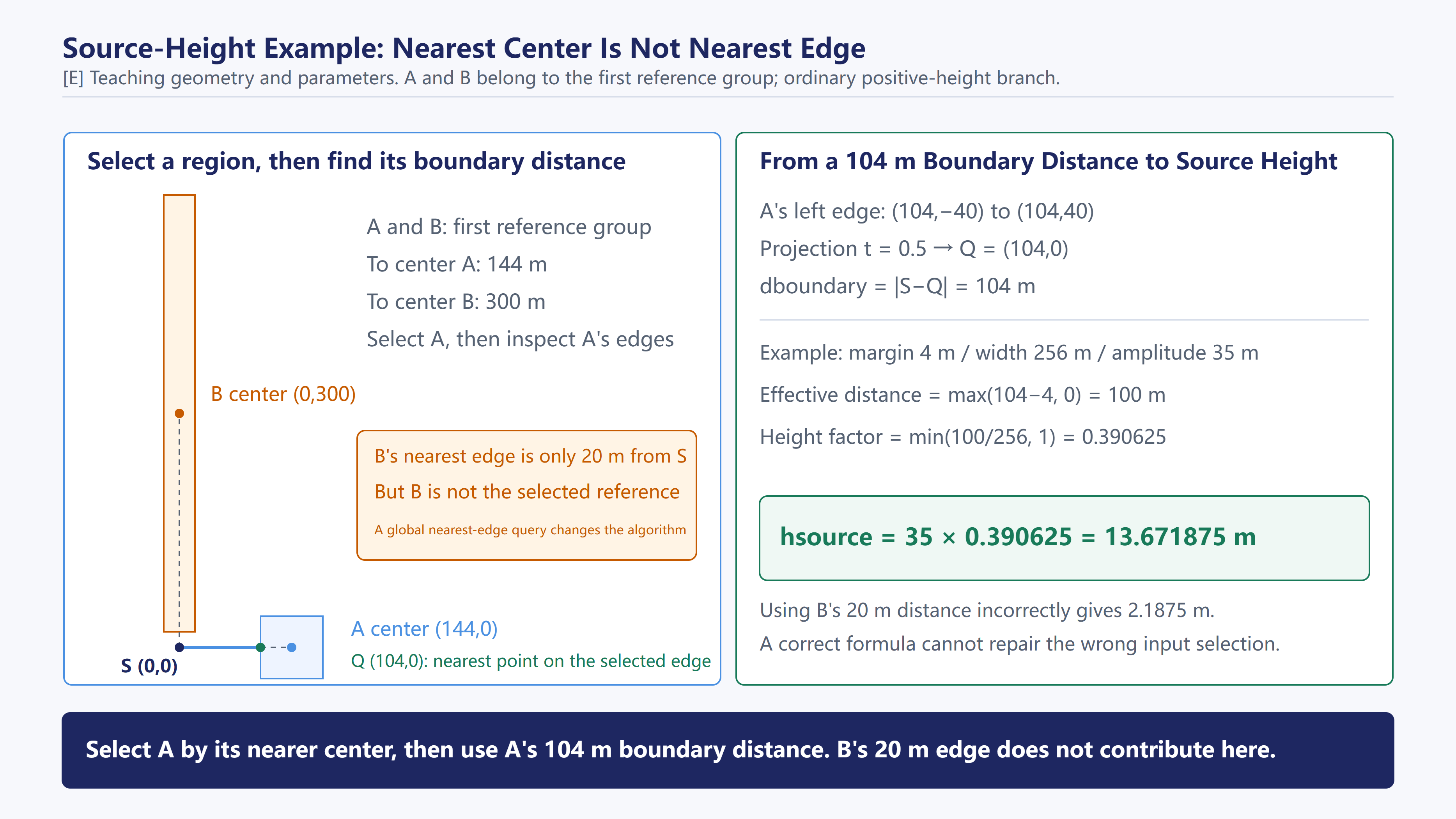
Figure 9: A teaching example. Select A by center distance, then find its nearest edge. The right side continues through effective distance, transition factor, and source height.
After selecting A, measure from S to all four edges. The left and right distances are 104 m and 184 m. Perpendicular projections onto the top and bottom edges lie on their extensions, so they clamp to (104,40) or (104,−40), giving sqrt(104²+40²)≈111.4271 m. The left edge therefore wins, with a boundary distance of 104 m.
Let the left endpoints be U=(104,−40) and V=(104,40). In the projection formula, V−U=(0,80) and S−U=(−104,40). The dot product is 3200 and squared edge length is 6400, so t=0.5. The nearest point is Q=(104,0), hence d=|S−Q|=104 m. Reference region, edge, projection, and distance are now determined.
Candidate priority is implicit here. Both A and B belong to the first reference-group type, so a closer center in the second type would not enter this search. Only an absent first type permits the second; both must be absent to enter the existing random fallback. That selection depends on current random state and is outside this example.
Endpoint handling matters for segment distance. In another teaching example, a segment runs from (0,0) to (10,0) and the query point is (14,3). Projection onto the infinite line gives (14,0), distance 3. Clamping to the segment gives endpoint (10,0), distance 5. Omitting the clamp gives incorrect boundary distances near polygon corners.
The denominator is the squared edge-vector length, so degenerate edges require defined handling. The ordinary formula here covers nonzero-length edges. A zero-length edge must not propagate infinity or NaN into minimum-distance and blending operations. Whether the current region generator can produce degenerate geometry depends on its input-validity constraints.
What Margin, Width, and Amplitude Change
Continue with source S and selected region A. Set margin to 4 m, transition width to 256 m, and amplitude to 35 m in the ordinary positive-height branch. Subtract the margin: max(104−4,0)=100 m. Normalize: min(100/256,1)=0.390625. Then hS=35×0.390625=13.671875 m. Incorrectly using B’s 20 m edge distance gives 35×(20−4)/256=2.1875 m. The paths already differ in reference selection; subsequent smoothing does not remove that computational distinction.
Holding these three parameters fixed while varying distance to the selected boundary separates the low, rising, and saturated ranges:
| Boundary distance d | After subtracting 4 m margin | Clamped height factor | Source height |
|---|---|---|---|
| 0 m | 0 m | 0 | 0 m |
| 4 m | 0 m | 0 | 0 m |
| 104 m | 100 m | 0.390625 | 13.671875 m |
| 260 m | 256 m | 1 | 35 m |
| 400 m | 396 m | 1 | 35 m |
This table describes the ordinary branch’s distance response. Movement in an arbitrary world direction need not encounter these values in order, because the selected reference region may change. The table isolates margin, transition width, and amplitude.
At S’s 104 m boundary distance, change one parameter at a time. Increasing margin from 4 to 20 m gives 35×84/256=11.484375 m. Restoring margin to 4 m and increasing width from 256 to 512 m gives 35×100/512=6.8359375 m. Restoring width to 256 m and increasing amplitude from 35 to 70 m gives 70×100/256=27.34375 m. These changes respectively move the start of the rise, alter its horizontal span, and scale its vertical extent.
A single mountain-strength parameter that changes all three would obscure the distinction between greater relief and a narrower transition.
Internal data may store amplitude normalized by a height scale. The source calculation discussed here uses a scale of 512, so division by 512 can be a vertical unit conversion. The 512 in the weight formula is instead a horizontal influence range. Identical numbers do not imply identical parameters or justify changing both with world extent. For S, normalization by 512 m gives amplitude 35/512=0.068359375 and source scalar 13.671875/512=0.026702880859375. Corner blending must keep all height terms in the same units. The examples below use meters for readability.
What Zero and Negative Values Preserve
With the first reference-group type present, margin and nonnegative clamping establish a low baseline in the ordinary source branch. Other conditions may set a source to zero. A specific branch without the first reference-group type also changes signs, allowing negative sources. Different sources can therefore contribute in different vertical directions.
Zero sources can constrain nearby heights toward low ground; negative sources can lower the weighted result, and positive ones may raise it. These describe numerical behavior, not fixed meanings such as canyon, summit, or lakebed. Actual landforms emerge from multiple sources, corner classifications, and smoothing.
Fallback rules for missing reference groups also matter. They select from a valid parent set, so both reference groups being empty differs from the entire parent set being empty. The first has a known fallback; the second involves invalid input or other handling. The random fallback cannot select from an empty parent set.
Distance Weights Blend Sources into Corner Heights
[D] The parameters 512, 96, and 10, negative-distance weights, and self term belong to the construction and blending path discussed here. [E] Values such as 20 m and 0 m explain denominators and normalization; they are not this request’s fixed configuration.
For corners entering general blending, the algorithm measures distance to each location center and, where applicable geometry exists, subtracts the configured envelope-distance parameter. This distance controls source attenuation and must not be confused with distance to a reference-region boundary in the preceding section.
Let d be the adjusted source distance. The current construction path first calculates source weight as follows:
d < 0:          w = 1000
0 ≤ d < 512:    w = (1 − d / 512)^6
d ≥ 512:        w = 0

If d < 96, then w = w × (1 − d / 96) × 10.
The parameters 512, 96, and 10 belong to this path. The distance range controls reach, the sixth power causes rapid attenuation, and the near-distance factor strengthens nearby sources further. Negative distances receive a strong weight; the branch must not be rewritten merely to make its curve continuous.
Corners also have a self-height term and self weight. In the ordinary nonnegative-distance branch, self height depends on distance and configured width. Self weight is increased in the near range and equals 1 outside it. The negative-distance branch uses a strong weight without adding a self-height numerator.
The final relationship is:
N = Σ(wSource × hSource) + selfHeightNumerator
D = Σ(wSource) + wSelf
hCorner = N / D
One corner class is set directly to zero according to its height group, bypassing general blending. These classification branches and normalization preserve low, flat areas, while surrounding corners form transitions.
A zero-height source can still change terrain. Two equally weighted sources at 20 m and 0 m blend to 10 m. The second adds nothing to the numerator but increases the denominator. Removing it raises the result to 20 m. Zero height therefore does not mean exclusion from calculation.

Figure 10: An equal-weight example illustrating normalization, without the actual corner’s self term or complete branches.
Gently sloping ground can be constrained directly by classification, produced by weights of zero-height sources, or extended through distance transitions from reference boundaries. These mechanisms must remain distinct to preserve both low areas and continuous slopes.
Two Distances Describe Two Spatial Relationships
Source height is computed from the source position and reference structure, then reused by multiple corners. Source weight must be recomputed for each corner because the same location influences nearby and distant corners differently. Storing a source height as one scalar does not restrict its effect to one position.
Subtracting the geometry-envelope parameter from center distance may produce a negative value, indicating that the query lies inside the range defined by this distance rule. The envelope parameter is used only as the confirmed radial offset; it is not necessarily the physical radius of a building’s outer wall. A location with multiple support shapes may have no single circular boundary.
Subtracting an offset also shifts the entire influence curve. With center distance 120 m and radial offset 40 m, weighting uses 80 m, inside the near-enhancement range. With zero offset it uses 120 m. Even unchanged location position and height can therefore exert different constraints on the same corner.
[E] Connect source S from the previous section to corner blending. S remains at (0,0) with height 13.671875 m. Add zero-height source T at (−128,0). Both radial offsets are 0. Corners C₁=(128,0) and C₂=(256,0) both use general blending. Their already-computed self terms are set to height 5 m and weight 1. This example does not derive those self terms from their separate distance and configuration calculations.

Figure 11: Continuing the source S teaching example. C₁ and C₂ share source heights and self terms; only corner positions differ. Displayed decimals are rounded.
C₁ is 128 m from S and 256 m from T; C₂ is 256 m from S and 384 m from T. All four distances are at least 96 m, so they use sixth-power attenuation without near-distance enhancement. Apply the same weight function and accumulate numerator and denominator terms:
| Term | C₁ | C₂ |
|---|---|---|
| Source S weight | (1−128/512)^6 = 0.177978515625 |
(1−256/512)^6 = 0.015625 |
| Zero source T weight | (1−256/512)^6 = 0.015625 |
(1−384/512)^6 = 0.000244140625 |
| Numerator N | wS×13.671875 + wT×0 + 1×5 = 7.4333000183… |
wS×13.671875 + wT×0 + 1×5 = 5.213623046875 |
| Denominator D | wS+wT+1 = 1.193603515625 |
wS+wT+1 = 1.015869140625 |
| Corner height N/D | Approximately 6.227612 m | Approximately 5.132180 m |
Moving from C₁ to C₂ leaves S’s height at 13.671875 m and its 104 m distance to reference A’s boundary unchanged. Corner-to-source distance changes: as S’s weight falls, C₂ approaches the 5 m self term. Removing zero source T at C₁ leaves the numerator unchanged but reduces the denominator, raising the result to approximately 6.310217 m. The denominator effect of zero-height sources remains visible in this complete example.
This teaching chain stops at two corners, not final pixels. The next stage forms height-bearing triangles, rasterizes them, and filters the result. The full-map validation at the end examines the output after these later stages.
How Sixth-Power Attenuation Distributes Influence
Outside the near-distance enhancement range, the sixth power makes weights fall quickly. At 128 m, the base weight is approximately 0.17798; at 256 m it is 0.015625; at 384 m it is only 0.00024414. Contributions near the outer limit can remain nonzero, but are usually much weaker than those of nearby sources.
Within 96 m, a second multiplier further distinguishes distances. It is 10 at zero distance, 5 at 48 m, and approaches zero near 96 m. Combined with the base attenuation, the final weight must follow the piecewise rule.
The strict branch boundary matters: multiply by the near-distance factor when d<96, but skip that multiplication at d=96. Plotting this rule directly therefore reveals a discontinuity. Negative distances receive a strong base weight and then enter the near-distance multiplication, giving behavior different from the value at zero. This curve differs from common smooth kernels; replacing it with a Gaussian changes the algorithm.
Such details determine whether a reconstruction evaluates the same function. A new algorithm could choose continuous weights, but this implementation must first preserve the conditions, constants, and evaluation order. The parameter discussion here is limited to the ranges these branches actually define.
How the Self Term Participates in Normalization
Normalization also requires a positive denominator D. For valid finite distances under these branches, the self weight is 1000 below zero; it is (1−d/96)×10, strictly positive, for 0≤d<96; and it switches to 1 at 96 m. Source weights are nonnegative, so this self term keeps the total denominator positive even without source contributions. This conclusion assumes valid inputs and the branches described here; it does not cover fallback handling for nonnumeric distances.
The corner’s self term enters the same numerator and denominator as the sources. Its height cannot simply be added after mixing the sources. For example, take source heights of 20 m and 0 m, both with weight 1, and a self height of 5 m with weight 2. The result is (20+0+10)/(1+1+2)=7.5 m.
Averaging the sources to 10 m and then adding the 5 m self height gives 15 m. Averaging the source average and self height with equal weights happens to give 7.5 m for these particular numbers, but fails when the self weight changes to 3. All terms must be normalized together using their actual weights; successive unweighted averages are not a substitute.
In the negative-distance branch, the self term contributes a large denominator weight without a corresponding height numerator. This strongly lowers the result. Mathematically, it resembles a heavily weighted zero-height constraint, but its branch and source type differ from those of a source. Keeping the distinction helps preserve subsequent rules.
When all weights are nonnegative and each denominator term has a corresponding height, the weighted average lies between the minimum and maximum input heights. Treating a numerator-free self term as a zero-height contribution extends this useful check. If ordinary blending suddenly produces a height far above every source, check units, the denominator, signs, or nonnumeric propagation first: a nonnegative weighted average cannot create an arbitrary peak.
How the Corner Field Produces Gentle Ground
Gentle terrain can emerge through several paths. Some corners are set directly to zero, constraining low areas. Some zero-height sources suppress surrounding heights through large weights. Some positions receive only a small positive height because they are close to a reference boundary. Triangle interpolation and smoothing then connect these discrete conditions into a surface.
A gentle patch therefore need not come from a later flattening pass; it may already exist in the base-height construction. This explains why region structure and zero sources matter. Replacing the upstream process with positive noise and relying on location support to flatten platforms would change the shape and connectivity of large lowlands.
Rasterizing Height Geometry into a Floating-Point Field
Corner heights next enter the draw geometry. Region polygons can be organized into triangle fans formed by a center and their edges, allowing heights in continuous space to be evaluated through triangle interpolation.
In this example’s base draw path, the ordinary center height sums endpoint heights while traversing edges, then divides by the number of endpoint contributions. The center position is the average of edge midpoints. Specific corner flags change the selection of center or endpoint heights, so the center value cannot be described as an arbitrary polygon average.
For a pixel center P inside a triangle, let vertex heights be h₀, h₁, h₂ and barycentric weights be λ₀, λ₁, λ₂. The pixel height is:
h(P) = λ₀h₀ + λ₁h₁ + λ₂h₂
λ₀ + λ₁ + λ₂ = 1

Figure 12: A barycentric interpolation teaching example. A, B, and C have heights of 0, 10, and 20 m. At P=(2,3), weights of 0.5, 0.2, and 0.3 give a height of 8 m.
First determine weights from planar coordinates, then apply the heights. With A=(0,0), B=(10,0), and C=(0,10), the relation P=λ₀A+λ₁B+λ₂C gives 2=10λ₁ along X and 3=10λ₂ along Y. Thus λ₁=0.2 and λ₂=0.3, leaving λ₀=0.5 because the weights sum to 1. The three subtriangle area ratios give the same weights. Finally, h(P)=0.5×0+0.2×10+0.3×20=8 m. Position determines the weights, not the relative vertex heights. These are teaching coordinates; P is a query point, not an identified pixel in the actual raster.
This step converts relationships between discrete corners into per-pixel slopes. The base draw in this example contains two layers accumulated with ADD blending, each contributing within its own coverage to one floating-point target. Later Stamp blending must be handled separately; this does not imply that all height writes are additive.
Pixel-center conventions must remain fixed. If a world position maps to a pixel corner in one stage and a pixel center in another, sampling shifts even when all vertex values are correct. World coordinates, draw coordinates, and texture row direction must also agree.
This stage retains R32 floating-point heights. Interpolation, accumulation, filtering, and local blending all occur in intermediate calculations; quantizing to 16 bits after every step would introduce repeated rounding errors. R16 conversion comes after the complete height composition.
The Triangle-Fan Center Must Follow the Draw Path
A polygon with n edges can form n triangles around a center. Each triangle contains that center and the two endpoints of one edge. Boundary heights remain on the original polygon while the interior connects them through the center. Changing the center height changes slopes throughout the polygon even if every boundary corner stays fixed.
The ordinary center position is the average of edge midpoints. If a closed polygon is traversed correctly, each vertex enters through its two adjacent edges, making this average equivalent in real arithmetic to the mean vertex position. It is generally not the area centroid: irregular shapes and uneven edge density can put a simple vertex average and an area-weighted centroid at different positions.
Endpoint accumulation for the center height must likewise follow traversal and flag rules. In the current base draw path, a particular corner flag causes the last encountered flagged corner to overwrite the center height; edge endpoints have corresponding replacement branches. This is not an average of every flagged corner, and “center height” cannot be treated as a universal geometric property.
Order therefore affects geometry construction. Reordering ordinary sums may only change the final floating-point bits, but a last-flagged-corner overwrite can change the selected height itself. Preserve the generator’s edge order instead of sorting edges by coordinates during serialization.
From a Triangle to One Pixel
In the teaching triangle above, P=(2,3) has a height of 8 m. Move the query point onto AB and its Y coordinate becomes 0, so C’s weight also becomes 0. Height then varies linearly between A and B alone. For example, AB’s midpoint (5,0) has weights 0.5, 0.5, 0 and a height of 5 m.
Adjacent triangles sharing an edge and its endpoint heights produce the same linear height along that edge. Height values are continuous there. Their third vertices usually differ, however, so the gradient can still change. A surface without cracks is not necessarily smooth; filtering addresses these spatial changes next.
Coverage rules determine which triangles write boundary pixels. If both triangles accumulate along a shared edge, ADD blending can create a thin raised line; if both omit it, a narrow gap can appear. Beyond the barycentric formula, coverage conventions, viewport transforms, winding, and draw order must agree. A conventional renderer handles these in rasterization; a CPU implementation must preserve them too.
The two ADD layers can be illustrated numerically: if a pixel receives 3 m from the first layer and 2 m from the second, the target accumulates 5 m. If the second layer does not cover that pixel, its 2 m contribution is absent. A “layer” here is an actual draw contribution; drawing a complete polygon twice cannot still be counted as a single interpolation.
Mapping Pixel Centers to Texture Coordinates
The 4096² texture in this article samples pixel centers. The 4097² representation used in the series’ runtime article is a vertex grid including both endpoints: 4096 intervals of 0.5 m plus one final vertex also span 2048 m. Their sample positions differ.
| Representation | First X sample | Last X sample |
|---|---|---|
| This article’s 4096² height texture | xmin + 0.25 m | xmin + 2047.75 m |
| 4097² endpoint vertex grid | xmin | xmin + 2048 m |
A downstream vertex grid consuming this texture therefore needs explicit world-to-texture mapping, resampling, and edge-query rules. Matching array indices directly does not work. Copying the last row and column alone does not convert the representation either: interior vertices are also offset by half a cell from texel centers.
Let the map extend from xmin to xmin+L along X, with N pixels. Under the pixel-center convention, pixel i lies at xmin+(i+0.5)×L/N. Conversely, world position x maps to continuous pixel coordinate (x-xmin)×N/L-0.5.
Here L=2048 and N=4096, so the first pixel center is 0.25 m inside the boundary. Placing it on the boundary would shift sampling across the map by half a pixel, or 0.25 m. This may be inconspicuous on flat ground, but on a slope rising one meter per horizontal meter, the shift in a single direction can produce approximately 0.25 m of height error.
Along Y, image rows must have an explicit direction relative to world coordinates. Flipping an image for convenient viewing is separate from its stored row order. A correctly oriented image in a viewer does not verify world-to-array indexing.

Figure 13: World coordinates map to continuous texel coordinates before four neighboring samples are interpolated. The teaching values do not describe a particular actual location.
Multilevel Smoothing Connects Different Spatial Scales

Figure 14: Heights after two-layer rasterization and the base surface after multilevel smoothing. Both use actual stage data from the same central 1024×1024 m area and a fixed oblique orthographic projection to connect planar structure with the height surface.
The left view has already combined layer 0 and layer 100 into the height field; the right shows the smoothed base. Compare slope connections and smaller undulations at matching positions. Neither view includes later location support, natural Stamps, or location textures. These oblique views use the existing 256² display samples of the central area. Consult the earlier top-down views for detail as well; the display mesh is not the original 4096² raster resolution.
[D] The five sample weights, offsets, levels, and final blend expression correspond to the current filtering path. [E] The four heights in the bilinear example and the terrain-shape examples explain the calculations. [R] Stage views show actual output.
Triangle interpolation produces continuous heights, but local gradients still change along triangle and region boundaries. Smoothing uses filtered results at different resolutions to create broader transitions.
The current pipeline uses a separable five-tap filter: first along X, then along Y. In one direction:
Hfiltered(P) = Σᵢ wᵢ × Sample(H, P + offsetᵢ)
The five weights are approximately 0.055028, 0.244038, 0.401870, 0.244038, and 0.055028. Together with sample positions, they define the kernel. Sampling uses fractional offsets and bilinear filtering; averaging five adjacent integer pixels is not equivalent.
| Sample | Main-axis offset, in texels of this level | Weight |
|---|---|---|
| 1 | −4.30908 | 0.055028 |
| 2 | −2.37532 | 0.244038 |
| 3 | −0.5 | 0.401870 |
| 4 | 1.37532 | 0.244038 |
| 5 | 3.30908 | 0.055028 |
These offsets are relative to the incoming sample coordinates; the other axis also includes a half-texel offset. Preserve the full-screen sample coordinates, offsets, and boundary handling together. The apparently asymmetric numbers are not a reason to recenter the kernel.
Starting with the 4096² floating-point field, the pipeline successively downsamples to 2048², 1024², and 512², applying the corresponding filters at each level. A lower-resolution texel spans more world space, so the same kernel smooths a broader spatial scale.
Although the final blend binds four levels, its current calculation directly samples only the 1024² and 512² levels back at the final resolution:
h₂ = Sample(H1024, uv)
h₃ = Sample(H512, uv)
Hbase(uv) = (h₂ − h₃) × 0.5 + h₃
In real arithmetic this is an equal-weight blend of the two levels. The implementation still preserves the single-precision evaluation order above. The 4096² and 2048² levels do not appear directly in the final formula, but contribute through earlier downsampling and cannot be removed.

Figure 15: This multilevel height filtering creates a continuous base field. It is separate from the Mip chains of static Stamp textures discussed later.
What One Bilinear Sample Reads
Let the continuous texel coordinate be (x,y), its lower-left integer coordinate (i,j), and fractional parts (fx,fy). For neighboring values h00, h10, h01, and h11, interpolate along X first, then Y:
a = h00 × (1 − fx) + h10 × fx
b = h01 × (1 − fx) + h11 × fx
h = a × (1 − fy) + b × fy

Figure 16: A bilinear interpolation teaching example with fx=0.25 and fy=0.5. Grid points represent texel centers. Compute a and b along the two rows, then blend by Y position. The diagram displays Y upward; actual sampling must still match texture row direction.
With samples of 0, 10, 20, and 30 m, fx=0.25 and fy=0.5 first give 2.5 m and 22.5 m, then 12.5 m. Each of the five filter taps may perform this four-value interpolation, so five sample positions do not mean only five input pixels are involved.
Neighboring taps may also overlap in the texels they cover. That overlap and the fractional offsets jointly define the filter response. Reading five integer indices and applying the same weights still produces a different result.
Why Half-Texel Offsets Belong to the Formula
The horizontal filter divides main-axis offsets by width and adds a half-texel offset on the other axis. The vertical filter retains its corresponding cross-axis offset. Read the offset table together with the incoming UV definition. The main-axis values alone suggest a kernel centered at −0.5, but incoming UVs, pixel centers, and the other-axis offset jointly determine the final sample positions.
Resampling is center-aligned too. When source width Ns is resized to destination width Nd, destination sample i maps to source coordinate (i+0.5)×Ns/Nd-0.5. Resizing 4096 to 2048, for example, maps the first output pixel to source coordinate 0.5, between the first two source pixel centers. Reading source index 2i instead biases sampling toward one side.
With clamp addressing, samples outside the texture remain at its edge instead of wrapping to the opposite side. Repeat addressing could mix right-edge heights into the left edge; zero padding would depress heights near the boundary. Filter weights, sample coordinates, and address mode jointly determine the result and must be recorded together.
How Lower Resolution Broadens Smoothing
A texel spans 0.5 m at 4096², 1 m at 2048², 2 m at 1024², and 4 m at 512². The same offset measured in texels therefore covers different world distances at different levels. A compact kernel can consequently process broader terrain scales.
The entire filter chain determines the final response. Lower-resolution inputs have already been filtered and resized upstream, so stage effects accumulate. A sharp boundary may spread slightly at high resolution, then enter a larger neighborhood through downsampling. Multiplying the last level’s offsets by 4 m alone does not establish the effective smoothing radius of the whole chain.
Separable filtering divides two-dimensional processing into horizontal and vertical passes. The first pass produces an intermediate field that becomes the second pass’s input. This reduces sample count, but does not allow both directions to read the unprocessed original and then average their results; that would omit the second filter’s effect on the first.
Which Terrain Variations the Final Blend Retains
Blending the 1024² and 512² results provides an intermediate response between two already smoothed scales. The higher-resolution level retains more local variation; the lower-resolution level favors broader shapes. Their current combination forms the base surface for location support and later textures.
[E] In shape terms, smoothing usually lowers and broadens a narrow peak while more readily retaining the overall trend of a gentle slope. This illustrates scale behavior, not a substitute for the actual stage output.
Implementation consistency: Preserve fractional sample offsets, bilinear filtering, half-texel conventions, and clamp addressing. The five weights sum to approximately 1.000002 at their original precision; do not renormalize them. Retain the single-precision order
(h2-h3)×0.5+h3. Although(h2+h3)×0.5is equivalent in real arithmetic, its rounding path can differ.
These small differences usually leave visible mountain structure unchanged, yet may cross a code boundary during final R16 quantization. Separating shape agreement from codewise agreement makes it easier to inspect terrain behavior and numerical details on their own terms.
Location Support Establishes Targets for Local Ground

Figure 17: Base height and the result after geometric location support on the 3D disk. All four stages share the same camera, lighting, color scale, and 625 m display radius, using actual stage data. The smooth disk-to-base transition is only a preview effect.
The left view already contains continuous hills and slopes; the right adjusts targets and transitions around locations on that base surface. Support acts locally, so the overall outlines usually remain similar. Read the calculations below and the later matching-coordinate markers to identify specific changes.
[D] The following sections explain supported target weighting, extent adjustment, and condition order. [R] The 84 circles and 0 rectangles are results of this request. [E] Parent–child heights and relief-coefficient examples use teaching values. These intermediate formulas do not yet constitute one closed-form function for every location.
Once the continuous base height is complete, location support is calculated before natural Stamps are drawn. Support therefore uses the base landform, without treating local texture detail that has not yet been added as input.
Location support includes position, horizontal orientation, geometric domains, and target heights. Local circles or rectangles transform into map space with their location instances, defining where to query and adjust the surface. They describe support extents; later height textures provide the detailed shapes inside each location.
Support targets come from queries of the base height field and cannot all be reduced to one sample at the location center. Ground variation over the domain, location configuration, and related instances may participate. For parent–child locations, a conditional weighted step incorporates child heights:
reference average = (self reference height + Σ child weight × child height)
                    / (1 + Σ child weight)
This expression summarizes only the weighting step. Region height overrides, configured offsets, parent–child target connections, and neighborhood limits may follow. Different locations take different branches. The average is an intermediate value, not necessarily the final support target.
Support applies the target height, domain, and transition to the existing field. It can raise or lower the surface. Its purpose is to connect local ground to location requirements, rather than add a fixed-shaped hill.
The circular support used here cannot be generalized to all natural Stamps. The current natural Stamps do not enter the same circle/rectangle support branch. Both eventually write height textures, but their preceding geometric processing differs.
Why a Domain Query Cannot Become a Center Sample
A location’s terrain requirements cover an area. Suppose its center is 10 m high, one side rises to 18 m, and the other falls to 4 m. The center value alone does not capture the slope it spans. Domain queries provide local upper and lower envelopes so target and transition calculations can account for that variation.
An instance and its asset-local geometry jointly determine the domain’s world position. A local support circle may be offset from the resource origin; a rectangle also depends on orientation. Drawing one equal-radius circle around the location XY would lose internal offsets and relationships between multiple shapes. Here, 54 location height draws correspond to 84 support circles and 0 rectangles: one location can have several support shapes.
A domain query also does not simply mean averaging every pixel inside the domain. Current processing uses height queries and upper/lower envelopes, while target calculation has separate parent–child and configuration branches. Store envelopes, reference heights, and target heights separately to distinguish descriptions of existing ground from requirements for the next stage.
For example, the existing ground’s maximum height may constrain a transition extent without becoming the target for the entire platform. A target may instead come from parent–child weighting followed by a particular region override and offset. Each intermediate quantity has its own scope; calling all of them “location height” obscures their different uses.
How Parent and Child Heights Interact
Parent locations and their attached locations are spatially related. Choosing targets independently can create awkward height differences. The confirmed weighting step gives the self reference a weight of 1 and includes children that meet the conditions and have positive coefficients. A child failing those conditions must not be included merely because it is nearby.
In a teaching example, the parent reference is 12 m and two participating children are 8 m and 20 m with weights 0.5 and 0.25. The average is (12+0.5×8+0.25×20)/(1+0.5+0.25)=12 m. Excluding the second child gives approximately 10.667 m. Relationships, weights, and participation conditions all affect the intermediate target.
This coordinates values; it does not make parent and child locations strictly coplanar on the final surface. Region overrides, configured offsets, satellite-location connections, and proximity constraints may still follow. A region height floor can limit a result, but its correction did not trigger in the 54 support items examined here. These conditional branches are not mandatory steps for every location.
Order matters too. Averaging before adding a uniform offset generally differs from modifying selected children before averaging. Limiting each term by neighborhood constraints before averaging need not match limiting the final average. The teaching formula covers the confirmed weighted step; the full implementation uses intermediate values in branch order.
Transition Width and Height Strength Are Different Parameters
Support must transition between the target surface and the surrounding base. Distinguish how far that transition extends from how strongly it changes height at a given position. One controls spatial extent, the other the degree of height blending. They are not interchangeable just because both use floating-point coefficients.
One confirmed extent calculation uses support radius R, minimum height hmin, maximum height hmax, target T, and configured coefficients a and b:
t = min(log(1 + a × R), 1)
relief = min((max(hmax, T) − hmin) / b, 1)
k = (1 − t) + t × relief
Within this branch’s valid positive parameter range, t sets an interpolation fraction based on radius, while relief expresses height variation relative to the configured scale. The resulting k multiplies an outward transition-width term. It adjusts the expanded extent; k must not be labeled as final per-pixel blending opacity.
Consider the teaching case t=0.5. If relief=0.2, k=0.6; if relief=1, k=1. For the same unscaled width term, the former uses a smaller expansion factor. This explains the formula without assigning unverified physical meanings to a or b or deriving complete pixel weights for every support shape.
Height-draw strength has a separate source, including a combination of support-shape and location-wrapper coefficients. Keeping these two parameter channels distinct allows transition extent and adjustment strength to be controlled separately. Name each parameter after the calculation it actually enters.

Figure 18: The cross-section illustrates the mechanism. Expanded extent and height strength enter separate calculations; the curves do not establish a newly confirmed support kernel.
Why Support Parameters Also Affect Early Placement
Support needs surrounding space for its transition, so it is not entirely independent of placement. The confirmed early spacing check uses both footprints, positions, and orientations, together with support flags, coefficients, and global parameters, to determine required clearance. A candidate position is rejected when actual clearance is insufficient.
In an isolated numerical test requiring clearance 10, actual clearance 9 is rejected, while 10 and 11 pass this check. Changing support coefficients while holding footprints fixed also changes the required clearance. Early placement thus accounts for support spacing as well as geometric overlap.
This geometric clearance check does not mean the terrain is fully blended first and its final slope then tested. The former uses geometry and parameters; the latter would require height simulation or prediction. This article uses the confirmed spacing relationship without adding full slope simulation, entrance-grounding retries, or protected-core masks.
Finally, a support target is not the building root’s final Z. Support modifies the terrain that receives the location; location textures will continue writing afterward, and scene objects may have their own local offsets and grounding behavior. Applying one support target to every object would skip their separate data relationships.
Natural Stamps Turn Configured Resources into Local Landforms
[D] Candidate hierarchy, asset transforms, and sampling each have supporting path evidence. [R] The 1,253 instances, 24 texture keys, and before/after height fields are results of this run. Confirming selection output does not mean every resource’s HeightProgram and Blend has been reduced to one formula.
Natural Stamp candidates follow relationships among Region / SubRegion, ZoneItem, StampGroup, and StampInfo. Weights, ranges, placement rules, and overlap conditions have distinct roles at each level. Selection first establishes its configuration context, then produces instances; pooling every resource and sampling uniformly over the map would change the process.
Selected instances hold resource references, positions, orientations, and related data. One resource can be selected repeatedly at different positions. This run has 1,253 natural Stamp instances referencing 24 distinct height texture keys. These numbers describe this request, not a fixed budget or selection weights.

Figure 19: Candidate organization at left, the 24 texture keys referenced by this run in the middle, and 1,253 actual initial instance positions at right. Thumbnails are normalized individually; × denotes draw-reference count.
The atlas shows referenced shapes; the point plot shows instances. Multiple instances can use the same local shape. Atlas entries 10 and 12 are labeled ×322 and ×327, their draw-reference counts in this run. Those counts cannot be written back into configuration as sampling weights. Frequency depends on candidate organization, grouping, selection, and layout results.
A low-contrast thumbnail also does not prove an asset is empty. The atlas helps identify shapes; pixel ranges and draw effects require the resource and its parameters. Points at right show initial positions only, without rotated footprints or subsequent joint and grounding transforms. The next stage diagram shows how those positions become terrain.
Static textures provide local height shapes. Resource pixels can encode ridges, depressions, and irregular edges, then enter the map through instance transforms. A support circle describes a geometric domain but cannot replace those internal pixel details.
Drawing also requires asset-internal transforms. The initial placement matrix positions the whole resource, while joints and local transforms determine the actual terrain element’s pose. Existing terrain height also contributes to draw inputs. Initial XY and angle therefore do not provide all the information needed for final sampling.
For each covered destination pixel, the draw program maps it to a local resource sample position, reads the height texture, combines instance and material parameters into a height output, and writes it into the existing field using the current blend state. The interface can be summarized as:
local sample position = determined by instance, local transforms, and draw geometry
texture sample = Sample(static height texture, local sample position, LOD)
draw height output = HeightProgram(texture sample, draw parameters)
new height field = Blend(old height field, draw height output, blend state)
HeightProgram and Blend remain separate because different resources and branches cannot all be reduced to “multiply the heightmap by strength and add it.” Position transforms, pixel calculations, and target blending jointly determine terrain changes. Local results can be higher or lower than the existing surface.

Figure 20: The lower-left view already includes location support; the middle adds natural Stamps; the right is their difference. Changes over the central 1,024×1,024 m range from −2.586 to 8.499 m, displayed on a symmetric ±8.499 m difference scale.
The difference view shows what natural Stamps change. Large-scale base relief remains recognizable, while shorter ridges and local irregularities appear. Red indicates raised ground, blue lowered ground. Both signs occur, so this stage cannot be summarized as adding one positive hill per instance. These colors compare consecutive stages, not error against the reference.
The upper row divides the change into three interfaces: obtain shapes and parameters, combine instance and asset-internal transforms, then sample and blend into the current field. They determine what can be read, where it is read, and how existing ground changes. The lower row records the net result after all natural Stamp draws. At overlaps, red and blue changes cannot be assigned to individual instances without considering draw order. Location height textures have not yet been written; the next location section continues the same chain.
The Complete Mip Chain Participates in Height Sampling
When a texture is scaled or mapped obliquely onto destination pixels, one pixel may cover several source texels. The Mip chain supplies different resolutions, and the sampler selects levels according to the sampling footprint. Linear Mip filtering also interpolates between neighboring levels.
Supplying only the highest-resolution mip0 can produce different sampled heights even when its pixels are exact. Reconstruction must preserve the source resource’s complete Mip chain, level dimensions, and sampling behavior. Copying mip0 into a new texture does not make the other levels irrelevant.
This is distinct from base-height multilevel smoothing. Base smoothing processes continuity over the whole map; a Stamp’s Mip chain determines what one local resource supplies at different sampling scales. They occur at different stages and use different data.
What Selection, Instances, and Resources Store
| Layer | What is established here | What does not follow |
|---|---|---|
| Configuration selection | Candidate hierarchy, level-specific parameters, and this run’s instances | Fixed selection weights inferred from reference counts |
| Instance transforms | Planar position, orientation, asset-local transforms, and existing-terrain inputs | Initial placement matrix equals final draw matrix |
| Sampling | Static texture, Mips, UVs, and sampler | Keeping mip0 alone reproduces the result |
| HeightProgram | Draw-specific height output | One strength-multiplication formula for all resources |
| Blend | Writes under the current blend state | Every draw is commutative height addition |
Natural Stamp hierarchy determines the context in which a resource appears. Parent ranges constrain generation space, groups organize candidates, item weights participate at their own selection level, and overlap conditions constrain spatial relationships between instances. Each number must retain its level: parent extent, child weight, and final instance count cannot all become one random-strength parameter.
Resource records store reusable shapes and draw information. Instance records store the current selection, position, transforms, and related state. Two instances can reference the same texture yet look different because of position, orientation, scale, existing ground, and draw order.
This request produces 1,253 natural instances referencing 24 height texture keys; another seed produces 1,077 instances and 18 keys. These statistics show variation between requests, but do not directly give resource-selection probabilities. A group may generate several instances, a shape may be reused, and instances may overlap.
Visible hill count is not instance count either. Two neighboring instances can merge into one ridge, one texture may contain several peaks, and a depression may mainly reshape an existing slope without creating a separate visible feature. Trace instances and pixel contributions to explain the surface; counting bright spots is not a placement count.
Mapping World Coordinates to Local Textures
In a simplified case with horizontal translation and rotation only, let instance center be p, angle θ, and local point q. The world point is P=p+R(θ)q. Drawing a world pixel requires the inverse mapping q=R(−θ)(P−p), then conversion to UV using local geometry extents. This explains why merely displaying a rotated texture is insufficient to write heights.
Scale, asset-local transforms, and joint transforms require matrices to be combined under a defined convention. Matrix operations generally do not commute. Rotating around the resource origin before placing it on the map differs from translating first and rotating around the map origin. Row-major or column-major storage alone also does not specify which side vectors multiply on.
For example, rotating local point (10,0) by 90 degrees gives (0,10); adding instance translation (100,50) gives (100,60). Translating first to (110,50) and then rotating around the world origin gives (-50,110). The same rotation and translation data produce completely different positions when composition order changes.
Actual natural Stamp transforms also query existing terrain heights. An upstream height difference can therefore affect both the base field and local height adaptation before entering draw parameters. Final differences need not all originate in current texture pixels; upstream data can propagate through instance transforms.
Static Pixels, Decoded Values, and Final Heights in Meters
A 16-bit single-channel texture stores codes, not automatically meters. A sample of 32,000 establishes only its raw value. Resource decoding parameters, geometry transforms, and the height program determine what height it represents. The final map’s −500 to 500 m encoding range cannot be applied to every local asset without verification.
Colored asset thumbnails add another representation. Mapping each image’s own minimum and maximum to shades of blue makes its shape easier to read, but removes absolute relationships between resources. Equally bright thumbnails can have different raw code ranges, and the same texture can produce different world heights under different draw parameters.
Asset previews answer what shape is inside the texture; decoding answers what a sample means; stage outputs answer how high the current ground becomes. These questions use raw data, algorithm parameters, and stage height fields respectively. None can replace the others.
Why Mip Selection Changes Height
Suppose a 256² texture spans 32 m in world space. Its highest-resolution texels cover about 0.125 m, while destination pixels cover 0.5 m. One destination pixel spans approximately four highest-level texels along an axis, so the sampler may use a lower-resolution level. This illustrates sampling footprint; it does not assign one fixed level to every current resource.
Neighboring Mip levels are interpolated too. A continuous level of 2.25 can be understood conceptually as blending samples from levels 2 and 3 with weights 0.75 and 0.25. Each level still uses bilinear sampling internally. If only the highest-resolution pixels are available, this step lacks the correct data.
Preserve the Mip chain as resource content. Rebuilding lower levels from mip0 may use different filtering, boundaries, and rounding, so it need not reproduce existing levels value for value. Reproducing sampling requires the stored pixels and dimensions at every level, sampler configuration, and geometric sampling footprint.
In this example’s local combined result, including the full chain reduced RMS over a restricted central area from approximately 2.37 mm to 0.122 mm and substantially reduced larger local deviations. These statistics belong to a specific area and stage; they do not replace final full-map R16 statistics. They demonstrate the effect of sampling, not the addition of new mountain resources.
How Draw Order Affects the Final Surface
Two local draws can cover the same pixel. Independent constant additions commute in real arithmetic, but a later draw that reads old height or uses replacement, limits, or weights may change result when reordered. Even an approximately commutative path can retain last-bit differences from floating-point accumulation order.
Preserve the established instance and draw order. Sorting by resource key may reduce state changes, but requires an equivalence argument before it can be treated as a valid optimization. Location height textures specifically follow natural Stamps; this order determines which output becomes the next calculation’s existing ground.
HeightProgram and Blend identify interfaces within local drawing while preserving the responsibilities of different branches. Position-to-UV mapping, complete sampling, and stage order can be explained in detail. Pixel programs not yet reduced to resource-specific closed forms should not be replaced by a generic “add height” formula. Explaining how the complete pipeline connects does not imply that every resource shares one scalar operation.
Location Textures Add Local Shapes

Figure 21: Results after natural Stamps and after location height textures on the 3D disk. All four stages share the same camera, lighting, color scale, and 625 m display radius, using actual stage data. The smooth disk-to-base transition is only a preview effect.
Figure 21 continues the 3D comparison in Figure 17. The left includes base height, location support, and natural Stamps. The right adds location height textures, matching the stage shown by the independently generated disk at the opening. The close-up below uses instance #0 to explain the added shapes and height differences.
After natural Stamps, locations write their own static height textures into the ground. Resource relationships typically lead from a location candidate to a Level, then from a terrain Unit to a texture. Instance position and local transforms jointly determine where it is written.
The 54 location instances reuse 44 distinct height textures, with dimensions including 80², 128², 184², 200², and 256². Resource dimensions, world scale, and sampling relationships must be stored separately. Equal pixel dimensions need not imply equal physical extents, while different dimensions can serve similarly sized locations.
Earlier support established the connection to surrounding ground; these textures supply the location’s internal shape. Platform edges, local slopes, and depressions can come directly from static assets instead of being approximated by support circles.
Locations therefore affect height in two separate steps, with natural Stamps between them: derive support from the base surface and adjust the field, then write location shapes after natural detail. Combining them into one “POI flattening” operation loses their inputs and ordering.
Completing this stage only establishes that location height textures have entered the surface. Final building-root Z, prop grounding, and whether collision uses the same result are downstream consumption questions.

Figure 22: Upper-row circles and rectangles illustrate support roles only; the asset at right is an actual 256×256 R16 texture. The lower row shows a 128×128 m window around instance #0, “Shut down grinder”: height after natural Stamps, height after all location draws, and their difference. Each #0 marker indicates the same location center.
The close-up uses instance #0, highlighted in orange in the layout view. Atlas entry 01 appears enlarged in the upper middle; the lower row shows how actual ground at its position changes. The before view already includes natural Stamps. The after view gains clearer internal edges and local planar areas. Only after the static asset is transformed and drawn can its shape be related to these world-space structures; support circles alone do not describe them.
Three different scales appear here: 256×256 is the static asset’s pixel size, 128×128 m is the observation window, and 0.5 m/pixel is the source full-map sampling scale. This does not mean every location asset maps to ground at 0.5 m per texel. Asset world extent and instance transforms still determine UV mapping.
Net change in this window ranges from −3.258 to 2.083 m, shown on a symmetric ±3.258 m difference scale. It measures the location texture stage; prior support is already present in both inputs. The after view includes all 54 location draws, and neighboring locations may overlap the window. These statistics are therefore not an isolated draw of instance #0. The upper circles likewise do not represent #0’s actual support geometry: they explain responsibilities, while the real asset and stage differences explain shapes and changes.
Why Support and Asset Shape Need Separate Explanations
Support reads the base field and establishes local connections. A location texture carries a preexisting height shape. Support circles do not create every slope inside that texture, and the arrangement of 84 circles cannot reconstruct the pixels in 44 assets. Both refer to the same locations but solve different problems.
Their behavior also differs in what remains unchanged. Static asset pixels may stay fixed, while the world surface resulting from transformation, decoding, and blending need not preserve them point for point. A support target may shift the baseline, an instance transform changes correspondence, and blending determines how the asset combines with current terrain.
Reusing a terrain asset therefore does not copy a patch of land with fixed absolute world heights. The reusable content is a local resource and its conventions. Whether particular relative shapes remain exact depends on the draw rules; without supporting evidence, the whole location cannot be described as undergoing vertical translation only.
A new project’s asset specification could define core, transition, and interface zones to preserve internal shape, absorb edge height differences, and validate entrances separately. That is an additional design proposal. The confirmed mechanism here does not establish such a three-zone mask, so it is not part of this article’s verified algorithm.
Several Locations Can Affect One Observation Window
A cropped difference view around one location may also include support and texture contributions from nearby locations. Centering the image on the first location does not attribute the whole difference to it. Interpret the result using instance coverage and stage inputs and outputs together.
The direct stage difference is ΔH=Hafter−Hbefore. Positive values indicate raised ground, negative values lowered ground, and zero no net numerical change. This measures an entire stage’s net result. A rise followed by a lowering may leave a small net difference even though both draws executed.
Comparisons should share world extent, orientation, and units. Independently normalizing before and after colors can make substantial height differences look similar. A separate symmetric difference scale distinguishes raising from lowering. An atlas shows shape; a stage difference shows effect. Their color scales serve different purposes.
After location heights are complete, the terrain contains the corresponding local shapes, but the scene is not finished. Buildings, props, navigation, and scattering read heights and other data separately. Later articles can cover those systems; this one ends at delivery of the final height data.
Radial Blending Connects the Interior to the Surroundings
[D] The 620–680 m interval and smoothstep belong to the current outer-blend path; draw eligibility still determines whether an outer resource is rendered. [E] The 20 m interior and −2 m outer heights explain weights and are not measured outer inputs from this run.
The map’s surroundings use separate inputs and transition rules. This run begins final outer blending 620 m from the center and completes it at 680 m. The circular transition lies inside the square computational texture; their boundaries do not coincide.
For world pixel position P, map center C, and radius r, map distance into the transition interval and calculate a smooth weight:
r = length(P − C)
t = clamp((r − 620) / 60, 0, 1)
α = t² × (3 − 2t)
At r≤620, α is 0; at r≥680, it is 1; between them it follows the smooth curve. In the current ordinary blend path, the height relationship is:
Hblended = (1 − α) × Hinterior + α × Houter
The weight changes gradually at both ends rather than switching height abruptly at one radius. Actual evaluation still requires the selected outer resource and blend state; the transition weight alone does not determine final height.
The outer input need not contain complex mountains. Under the current default usage, an outer draw that fails eligibility leaves its target at the corresponding initial value. A resource existing, being referenced in configuration, and actually being drawn are different conditions. Determine the effective inputs for this run before blending.
What the Transition Does at Its Ends and Midpoint
Smoothstep α=t²(3−2t) is 0 at t=0 and 1 at t=1. Its derivative 6t(1−t) is zero at both ends. Weight change therefore does not begin or stop with nonzero speed at the transition boundaries. This improves the weight curve’s connection; it does not automatically make the two input heights or slopes match.
In a teaching case with constant interior height 20 m and outer height −2 m, output is 20 m at radius 620 m. At 650 m, t=0.5 and α=0.5 give 9 m; at 680 m the result is −2 m. At 635 m and 665 m, weights are 0.15625 and 0.84375, producing approximately 16.5625 m and 1.4375 m.
Both interior and outer heights contribute in the transition band. The outer contribution can be omitted only when that height is exactly zero. In general, sample both effective inputs and keep them in the same world-height units.
A Circular Transition inside a Square Data Domain
Radius depends on both horizontal components. Even when neither x nor y exceeds 620 m, sqrt(x²+y²) may do so. Point (500,500), for example, has radius approximately 707.1 m and is already beyond the transition. Independent X/Y thresholds would create a square with substantially different corner behavior.
Crop extent matters when analyzing the outer area. A central square may intersect the transition ring only at its corners; those corners do not represent the full circumference. Full-map views show overall transition shape, while radial statistics identify where errors begin. Label both observation scopes explicitly.
The outer target’s initial value is part of the effective input. When a draw fails this request’s conditions, the target can retain its initial state and still enter blending normally. Forcing distant mountains merely because the resource exists changes the algorithm. Choosing outer content for visual appeal does not replace request and eligibility rules.
Some other height operations build local rises from ring distances, while others blend two fields. Both involve radius without sharing a formula. This section covers final outer blending only; other radial adjustments are outside this stage.
Encoding a Deliverable R16 Heightmap
[D] Current encoding uses the range mapping and R16 UNORM output below. [R] Final statistics come from encoded files and do not substitute for intermediate floating-point errors.
After all height processing, the floating-point field converts to 16-bit normalized heights. First map the range:
u = clamp((Hmeters + 500) × 0.001, 0, 1)
Then convert to the output format:
q = UNORM16(u) // format conversion of the current R16 UNORM render target
The implementation used for final comparison writes mapped floating-point heights into a DXGI_FORMAT_R16_UNORM render target, whose output path performs float→UNORM16 conversion. The CPU reads back encoded two-byte pixels and saves them row by row without another floor or round call. UNORM16 explicitly identifies this format-conversion rules rather than substituting a language’s rounding function.
A separate CPU encoder would need to match clamping, scaling, rounding, and integer conversion, especially near half-integer boundaries. Saying “round to nearest” alone does not prove codewise equivalence. The final statistics here use the render-target readback files, not an approximate CPU encoding. Codewise comparison is limited to the saved output path and platform; changing graphics API, hardware, or CPU encoding requires rechecking boundary conversions.
Decode integer codes from 0 to 65535 as:
Hmeters = q × 1000 / 65535 − 500
This covers approximately −500 to 500 m. One code unit is approximately 0.015259 m, or 1.526 cm. Values beyond the range clamp to the endpoints and no longer have a linear representation.
Quantization allows very close floating-point heights to land on adjacent codes. Preserve single-precision constants, evaluation order, and UNORM conversion rules. Equality in real arithmetic does not guarantee equal codes after floating-point reordering.
Delivery must include world extent, resolution, coordinate direction, and decoding conventions alongside pixels. Downstream queries usually interpolate neighboring pixels. Without those conventions, a pixel file cannot identify where a world position should sample or how many meters it should return.
Why Residual Differences Can Stay within One Code
R16 maps continuous heights to 65,536 codes. Nearly identical floating-point values may straddle a quantization boundary and become adjacent integers. A somewhat larger difference may still lie inside one code interval and encode identically. Code agreement and floating-point RMS therefore measure different properties.
A code unit of approximately 1.526 cm does not mean every pixel has that error. Here, most codes match exactly and the remainder differ by one. Calling that unit the maximum difference is accurate; treating it as the average exaggerates the result.
Conversely, a small average does not rule out local defects. A few locations with one-meter errors could be diluted by millions of correct pixels. Record exact agreement, maximum absolute error, RMS, and a spatial difference map together, then inspect relevant local windows.
Pre-encoding clamping matters too. Inputs beyond approximately ±500 m saturate, so different out-of-range heights may produce identical codes. R16 agreement alone could hide that lost information without a floating-point range check. Heights in this example stay inside the encoding interval; encoding is not doing the main work of clipping terrain amplitude.
How Downstream Systems Read the Heightmap
Along with raw pixels, record horizontal extent, grid dimensions, row direction, height scale, and offset. Convert world points to UVs or continuous texel coordinates, query codes under the agreed rules, and restore heights in meters. Only consistent conventions align the terrain surface with downstream position queries.
With linear decoding and no additional nonlinear operation, interpolating codes before decoding and decoding samples before interpolation are equivalent in real arithmetic. Sampling precision and floating-point order still affect implementations, so exact matching requires a defined path. This is the basic mathematical relationship for consumption, not evidence that every downstream system has been individually verified.
One heightmap can also produce several downstream representations. Rendering may sample a vertex mesh, collision may build its own height structure, and previews may downsample to images. These conversions do not turn a low-resolution preview into the original final data suitable for centimeter-level evaluation.
Organizing the Implementation around Stage Inputs and Outputs
Each stage should have explicit inputs and outputs. Source-height calculation reads region relationships and planar location data, producing source scalars. Corner calculation reads sources and spatial distances, producing height-bearing corners. Drawing converts geometry into an R32 field; filtering produces continuous base height.
Support needs base heights and location geometry, producing support parameters and adjusted ground. Natural Stamp and location-texture stages read their respective instances, static assets, and current ground. The outer stage combines interior and outer inputs before R16 encoding. This structure makes data readiness checkable and helps prevent later heights from entering earlier calculations accidentally.
Name saved intermediates by content, such as “after support, before natural textures” or “after location textures, before outer blending.” “Second heightmap” loses stage meaning and makes mismatches easier. Descriptive names and numerical comparisons together make results reviewable.
This organization also identifies where changes belong. Large-scale terrain relationships belong in regions and sources; local shapes in resource and instance drawing; location connections in support; distant boundaries in outer blending. Adjust parameters at the stage responsible for their effect.
Results and Scope

Figure 23: All four large views show stage outputs over the central 1,024×1,024 m. Markers #0–#5 identify the same task-location coordinates in every column and match Figure 6. The third column’s small view shows net stage change; the others show reference heights. Millimeter statistics cover the inner 400 m, a different scope and data type from the final full-map R16 comparison below.
Follow #0, “Shut down grinder,” across the columns to connect the task input to one terrain position: base ground, location support, natural Stamps, then location height textures. Figure 22 enlarges the final step at that location. #1 is another instance of the same task type; #2, #3/#4, and #5 correspond to organic soup, detector towers, and communications facilities. White markers are coordinate indices, not building outlines or support extents. Nearby height changes may still include other instances.
The columns show distinct contributions: base height supplies continuous hills, support adjusts local connections, natural Stamps add dense detail, and location textures add instance-specific shapes. Similarity between the first two columns does not mean support was skipped. At this scale, limited local changes are less conspicuous than natural textures and require differences and numerical checks.
The figure retains the recorded comparison scopes: inner-area RMS is 0.203 mm for base height and 0.122 mm after support. Natural Stamps have no independent stage reference, so that column shows before/after increments. The last column compares against the final reference inside 400 m, unaffected by later outer blending. Stage change, inner-area reference error, and full-map agreement use different measures.
Outer blending and R16 encoding still follow these four columns. Central views cannot cover the full transition ring, and floating-point stage statistics do not capture all final quantization effects. The delivered result therefore requires the full-map comparison below.
[R] This pipeline has generated a complete 4096² R16 heightmap for one fixed tundra request. Against its corresponding reference, 16,742,045 of 16,777,216 pixels match exactly, or 99.7904%. Every remaining pixel differs by exactly 1 code. Converting the final code differences under the current −500 to 500 m mapping gives full-map RMS of approximately 0.699 mm and a maximum absolute difference of 1 code, approximately 15.259 mm. These measure the final deliverable, not identical errors at every intermediate floating-point stage. 99.7904% is pixelwise agreement of final R16 codes, not a visual-reconstruction score or average accuracy across other seeds or biomes.
Formally, use Δq=qgenerated−qreference and ΔH=Δq×1000/65535, then take the square root of the mean of ΔH² over all pixels. Most Δq values are zero, with only a small fraction at ±1, so RMS can be much smaller than one code unit. RMS describes overall differences; maximum absolute difference describes the extreme.

Figure 24: Both heightmaps share one color scale. Each displayed difference block retains the maximum absolute code difference among its 4×4 original pixels; statistics use full resolution. Colors show height, not surface materials. RMS describes final R16 code differences decoded to meters over the full map.
High agreement comes from preserving inputs and conventions across the whole chain: region relationships, draw order, filter coordinates, complete Mips, local resources, outer inputs, and encoding all contribute. A change can affect codewise comparison without visibly changing terrain. Current data establishes residual differences within ±1 code. This is consistent with small floating-point differences crossing quantization boundaries, but the final histogram alone cannot attribute every differing pixel to rounding. Corresponding pre-encoding floating-point values are needed to distinguish causes.
This result validates height output for one request. A second seed has produced natural Stamp output, but lacks a corresponding reference and the same complete location-texture stage. Other biomes, all location-layout branches, resource runtime lifecycles, and complete scene content require separate validation. This article explains the stage structure and established formulas without filling unconfirmed branches with universal rules.
AI Collaboration Retrospective
AI assisted with organizing configuration relationships, formulas, stage results, and figures. Human checks focused on data roles and stage order: zero height versus zero weight, geometric support versus pixel shape, base filtering versus resource Mip chains, and completed height output versus a completed scene.
The article follows the algorithm’s inputs, calculations, and outputs. Reported results come from saved generated data, with the final R16 files checked again during preparation. Explanatory diagrams and teaching examples were not treated as new terrain experiments.
Part II, Rebuilding POI, Stamp, Vegetation, and Rock Layouts from the Original Algorithm follows task requirements into location candidates, positions, and orientations, then examines how vegetation, rocks, and block-based Scatter use resource and terrain data.
Surface Layer generation needs a separate explanation: configuration and spatial conditions produce coverage weights or masks for the material system. The height colors here show relief; they do not demonstrate reconstruction of surface materials.
5 thoughts on “Procedural Terrain Reconstruction, Part I: Rebuilding Heightmaps at True Scale from the Original Algorithm”