
This series examines secondary motion on animated characters. Base animation determines how the body walks, runs, and stops, while skeletal constraints and dynamic solvers continue to adjust the local pose. We follow animation sampling, bone transforms, state updates, and skinning to explain what each stage reads and how to check its output. This first article covers chest and hip helper bones. The next follows the cloth and ponytail as they respond to the body.
Chest and hip helper bones provide a useful view of how authored animation interacts with dynamic simulation. During walking and running, the pelvis, spine, and arms continuously change their target poses. Sprinting, releasing the movement input, and stopping change the targets’ speed and direction again. Lag, rebound, and corrective deformation emerge throughout this process. We need both the moving targets and the previous positions and velocities to explain the output, so the reconstruction retains continuous results for steady gaits and transitions.
As the character transitions out of a sprint, the legs begin changing animation while the chest and hip helper bones still respond to the preceding motion. We reconstructed a character from a third-person action game in Blender, preserving the transitions between walking, running, sprinting, input release, and stopping. The two close-up views below show the stop. Watch the torso decelerate, then follow the local response.
Contents
- Source animation sampling and helper-bone updates
- Component space and parent-local space
- Fixed-time-step simulation for helper-bone springs
- BtoB correction from upper-limb distances
- A display-aligned comparison of 30/60 Hz pose input
- Separating base-animation and procedural displacement
- Animation input and transition timing during a sprint stop
- Left-foot stop correction and downstream pose input
- Bone writeback and original-instruction comparison
- Reproduction workflow and source entry points
- Additional animation clips
- From body pose to secondary motion
- AI collaboration retrospective
Both views show the same solved motion at half speed. The front-quarter view on the left includes the torso and arms. The tighter rear view on the right follows the hip silhouette. Both use the same evaluation times.
Source animation supplies the chest and hip helper bones with a target pose each frame. A rotation constraint is applied to the chest first. The spring then updates translation using its retained position and velocity. After the spring update, a corrective stage named BtoB reads the component-space relationship between the chest and upper limbs and adjusts the chest’s local transform.
The displacement visible in the final image includes base animation, spring motion, and subsequent correction. The diagrams identify what each stage reads and modifies. The stop comparisons then help locate the first stage at which a change appears.
This is an offline Blender reconstruction using the source skeleton and character assets. Animation tracks and configuration establish the inputs. Replaying original executable instructions with specified inputs checks individual calculations. Continuous animation and rendered footage show the stages working together.
The game’s runtime input history, complete state machine, full PBIK implementation, and bone and skinning submission order still require in-game verification. The article ends with a left-leg stop correction to show how the body pose reaches downstream systems. Cloth and ponytail simulation continue in the next article.
The implementation begins with coordinate spaces. The solver tracks targets in component space, then converts its output into a local pose using the current parent transform. We then examine fixed substeps, velocity history, and the frequency of external pose inputs, followed by controlled comparisons of the chest rotation constraint and BtoB correction.
Watch the motion first, then refer to the coordinates and formulas. Walking and running loops show the response within a gait cycle. Stopping shows how spring state survives an animation change. Technical overlays expose target and integrated positions. The 30/60 Hz comparison shows the effect of changing pose-input frequency, while the spring and BtoB toggles show how their respective stages affect the image.
Source animation sampling and helper-bone updates
The project reads local QTS transforms—quaternion rotation, translation, and scale—from the body and head animation data, together with the parent indices. At each output time, it evaluates the body pose and uses that pose to update the helper-bone targets. The four nodes examined here are the right hip Ab-R-Hip-Reg, left hip Ab-L-Hip-Reg, left chest Ab-L-Breast, and right chest Ab-R-Breast. The chest rotation constraint also reads the same-side Dm-*-Breast-Point. These names identify nodes in the source skeleton. Similar names, nearby positions, or a shared region of the visible mesh do not establish a parent-child relationship. Transform calculations must use the parent indices and bind pose.

Several different positions can describe the same shoulder, hip, or chest region along this chain. The bind pose defines reference axes and orientation. Source animation supplies the current frame’s transforms. The chest constraint updates rotation. The spring maintains its own integrated position and velocity, and the exported pose also passes through BtoB. For the right chest bone, the spring target and final written position can therefore differ within the same frame. Identify the stage behind each value before subtracting them.
| Data | Source and lifetime | What it explains |
|---|---|---|
| Reference bind pose | Read from the asset and retained for the sequence | A bone’s reference axes and orientation offset relative to its reference target |
| Source pose | Resampled and blended at each evaluation time | Where base animation places the body and helper bones this frame |
| Constrained pose | Computed from the current source pose | How chest orientation follows the same-side target |
| Spring state | Retained across frames and animation segments | How position and velocity evolve under the current target |
| BtoB correction state | Updated from the current pose and retained history | How the local chest transform changes as the upper limbs approach |
| Final local bone matrix | Output for the current frame | The pose read by the skeleton and downstream cloth and hair systems |
Local animation can already contain tracks for the helper bones. When the torso pitches forward, the chest position in component space changes through its parent chain even with the spring disabled. Subtracting the static bind pose from the final pose combines every change along that chain. To isolate the spring contribution, align the time, node, and coordinate space, then compare continuous runs with and without the spring.
Combining body and head animation
Body and head tracks come from separate source data. Some bone names appear in both outputs, so the source of each shared transform must be checked to avoid applying it twice. Other head channels continue to use the head tracks. This matching takes place at the skeleton level. Verification must resolve individual bones, independently of textures, materials, or skinned-vertex indices. Matching bone counts alone is insufficient.
When evaluating tracks outside an animation graph, first resolve source bone indices to names and the original parent chain, then build a complete local pose at each time. For a subtree diagnostic, bones outside the affected subtree can retain the same base pose. This is especially relevant to the chest constraint, which reads the current target orientation. That target can inherit rotation from the body or another ancestor. Exporting only the target’s rotation curve loses the parent’s contribution to the current frame.
The character uses the green outfit, and the offline sequence retains the default combat pose. In the configuration, BS_Green_Suit references AdditiveBody_Type1 with a parameter of 0.4. An earlier fixed-weight experiment used that value. The current reconstruction disables the idle additive overlay (Idle Additive) according to the pose conditions and weight history, leaving the actual Type1 weight at zero across all 280 display samples. Keep outfit appearance, asset reference, and evaluated weight separate. Two recordings of the same outfit can use different overlays. Shoulder-strap differences and layered data from the earlier candidate cannot explain the current one.
If 0.4 is treated as a constant per-frame weight, the source chest and shoulder transforms change before the spring. The spring receives a different target trajectory, and BtoB may read different arm distances. The skinned result then differs even if integration, damping, time step, and bone mapping are correct. Check the source pose and active equipment-overlay weights before tracing downstream differences.
Component space and parent-local space
Bind poses and animation tracks can both represent each bone relative to its parent. This article uses column vectors. A point is transformed by the child-local matrix first, then by the parent’s component matrix. For bone i in the current frame, Lᵢ is its local matrix and Cᵢ its component matrix; p denotes the parent. A root has no parent, so its component matrix is its local matrix.
// C: component-space matrix. L: local matrix relative to the direct parent.
// A root has no parent, so use its local matrix directly.
C_root = L_root
// Column vectors: apply the child-local transform before the parent transform.
C_i    = C_parent · L_i
Position can be read from the translation column of Cᵢ. To compare bone rotations, extract rotation using the project’s convention and ensure that reference and current rotations use the same coordinates. With scale present, the entire 3×3 block is not necessarily orthogonal and cannot simply be transposed as an inverse. The transpose in the chest formula applies to a rotation basis. Preserve meaningful signs in the source local scale when reading transforms back.
Component space has two advantages here. Targets and integrated positions share the same axes, so their error vectors can be subtracted directly. The hips, chest, and arms also share a space for distance calculations. Later animation evaluation and skinning still require local bone matrices, so the result must be converted back using the current parent transform.
// C_i is the original component matrix; C'_i is the corrected result.
C'_i = replaceTranslation(C_i, solvedPosition)  // Retain rotation and scale.
// Convert the corrected pose back into the current parent's local space.
L'_i = inverse(C_parent) · C'_i

Consider a 2D example. Rotate the parent 90° around component Z. Its local +X now points along component +Y. With no parent scale, a requested 1 cm displacement along component +X must be written along local −Y. Adding it directly to local +X would make parent-chain composition rotate that displacement into component +Y. The magnitude can be correct while the direction is wrong. Drawing the parent-local axes, component axes, and displacement arrow makes this easier to diagnose than three printed floats.
Nonuniform scale introduces another conversion. If a parent axis is scaled by two, a 1 cm component-space displacement along that axis needs half a unit locally. Inverse rotation followed by componentwise division by parent scale helps explain a shear-free translation, rotation, and scale (TRS) transform. The writeback formula uses the inverse parent component matrix because the entire transform participates. This derivation does not establish lossless quaternion-and-scale decomposition for arbitrary matrices containing shear.
If a stage modifies a parent before its descendants, those descendants must use the updated parent matrix. If their own local tracks are to remain unchanged, the next forward-kinematics pass can propagate the new parent pose naturally. Diagnostics should distinguish a written descendant-local transform from a changed descendant-component transform. Both observations may be valid at once.
Writing component-space results into the local pose
The pseudocode below follows Figure 2’s column-vector convention. Inputs belong to the same frame, and the parent matrix must be invertible. A component-space displacement requires a direction-and-length conversion. A corrected full component matrix requires a relative-transform calculation. Choose the path that matches the input.
// Column-vector matrices: component = parentComponent × local
parentInverse = inverse(parentComponent)

// A. Input is a component-space displacement Δp_C.
// Use the linear part; parent translation does not affect a displacement.
deltaLocal = linearPart(parentInverse) * deltaComponent
localAfter = localBefore
localAfter.translation += deltaLocal

// B. Input is the corrected full component matrix C_after.
// componentAfter contains the complete corrected component transform.
localAfter = parentInverse * componentAfter

// To replace component translation only, B can receive:
// componentAfter = copy(componentBefore)
// componentAfter.translation = solvedComponentPosition
Path A uses the inverse matrix’s linear part so that parent position is not added to a displacement. With the unscaled +90° parent in Figure 2, (+1, 0, 0) cm becomes (0, −1, 0) cm locally. Path B uses the complete inverse because both position and basis must be expressed relative to the parent. Both paths need the parent matrix from the current evaluation stage.
Execution order of chest rotation and translation
The chest helper bone first computes a reference orientation offset. For one side, read the reference component rotations of the same-side target Dm-*-Breast-Point and the helper bone. Inverse reference-target rotation expresses the helper’s reference orientation in the target’s axes. The current target rotation then brings that offset back into component space.
// Express the helper's reference orientation in the same-side target's axes.
R_offset = transpose(R_ref_target) · R_ref_bone
// Bring the reference offset into component space with the current target.
R_new    = R_current_target · R_offset
Copying the target’s current rotation assumes an identity reference offset. The helper still follows the target, but its resting orientation changes. For a same-axis example, a 10° reference target and 25° reference helper imply a 15° offset. If the target reaches 40°, the output should be 55°. Writing 40° directly loses that 15° relationship. General 3D rotations cannot be composed by adding Euler components, so the formula preserves matrix multiplication order.
This constraint retains component translation and per-axis scale, then converts the new rotation back to local space. The following spring stage updates translation. If chest orientation differs between videos, first check the target bone, the reference pose used for the offset, and the current parent used for inversion. Comparing target and integrated positions is then necessary to attribute translation to the spring. The hip translation spring also does not actively solve pelvis rotation.
Fixed-time-step simulation for helper-bone springs
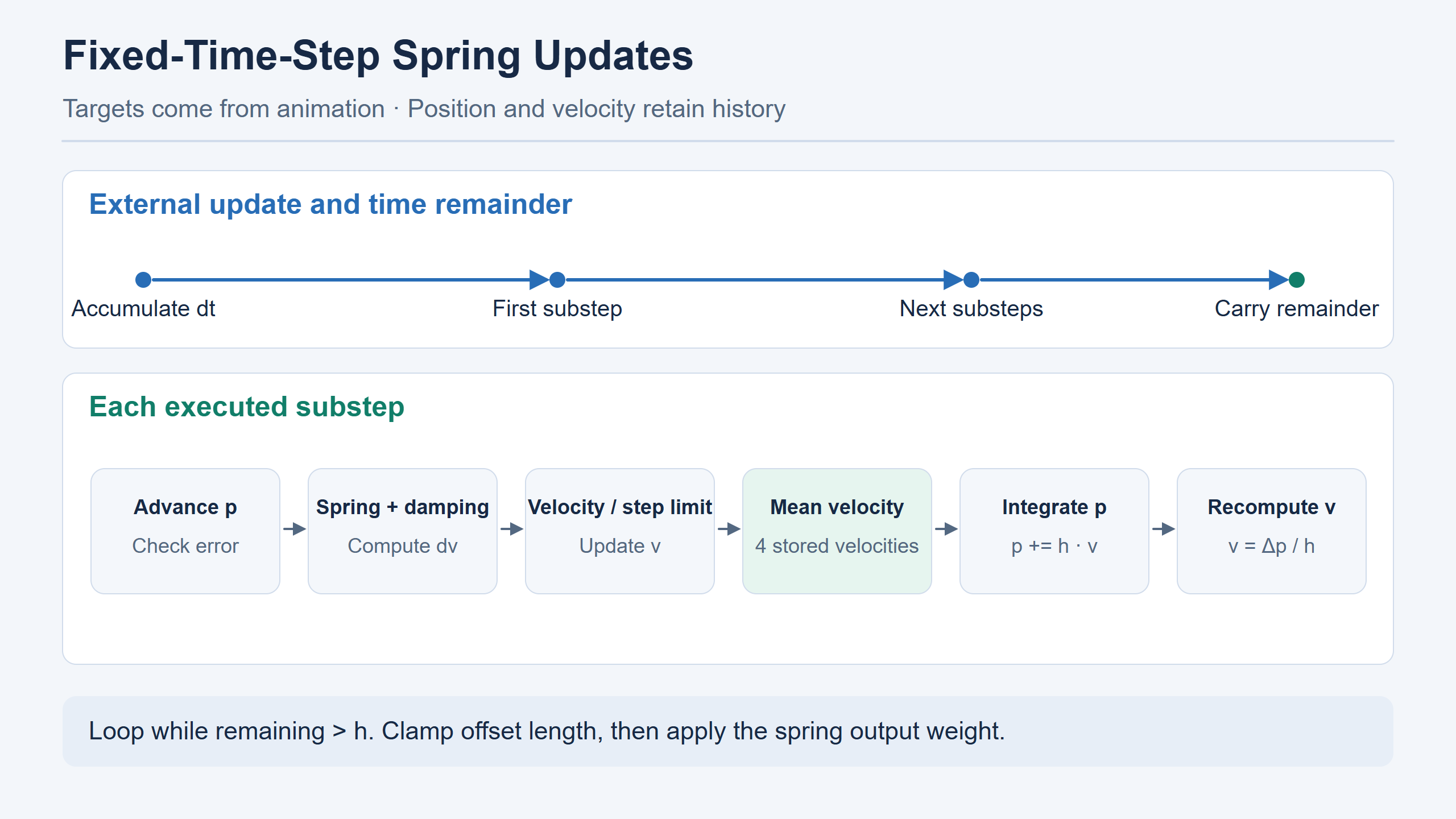
Numerical integration advances velocity and position in small time increments. A fixed time step keeps the duration of each internal update constant; each such update is a substep. The solver accumulates the external frame time, executes the corresponding substeps, and carries any remaining time into the next frame. The velocity-history buffer stores a fixed number of recent samples and overwrites the oldest when full.
Base animation supplies target position x. The spring stores integrated position p, velocity v, unprocessed time, and a ring buffer of velocity history. When the source animation changes, x comes from the new blended pose while p and v carry over. Even identical target positions can yield different outputs if one state is accelerating toward the target and another has just overshot and is decelerating. This retained history adds lag and rebound to the source pose.
All four nodes in this reconstruction store component positions in centimeters and use stiffness 400. Left and right bones of each region share parameters but update independent states. Asymmetric animation can supply different targets and produce different offsets from the same settings. The table lists the candidate configuration. Supplied integration inputs and parameters recovered from the source data must be recorded separately.
| Parameter | Hip helper bones | Chest helper bones | Role in the update |
|---|---|---|---|
| Stiffness k | 400 | 400 | Multiplies the target-to-integrated-position error vector |
| Damping d | 25 | 20 | Subtracts the velocity-dependent damping term from the restoring term |
| Maximum offset | 2 cm | 1 cm | Limits the integrated position’s distance from the current target |
| Velocity-history length | 4 | 4 | Averages recent velocities inside each substep |
| Error-reset threshold | 255 | 255 | Uses the same units as position. Above the threshold, snap position to the target and clear velocity. |
| External inputs | Time factor 1, zero extra velocity, output weight 1 | Same | Inputs used for this reconstruction |
Stiffness converts positional error into a restoring term. Damping contributes deceleration. Maximum offset limits the final target-relative displacement. These settings interact. Chest damping is lower, but so is its offset limit, so either parameter alone cannot predict the visible amplitude. Compare target trajectories, velocity histories, and final offsets from the same segment. Left and right source animations are also not synchronized mirror images; retain bone names in the records.
Accumulating frame time and executing substeps
At an external update rate of 30 Hz, one frame represents about 33.3 ms. The spring advances in increments of about 8.33 ms, or 1/120 s. Each internal update is a substep. A frame typically executes about four substeps, with each one continuing from the previous position, velocity, and history. Four is an illustrative time-scale comparison: the actual count depends on accumulated remainder, floating-point operations, and the strict loop condition below. Dividing frame time by step duration and rounding is not an equivalent implementation.
Substeps are internal solver updates, not additional animation or video frames. In this implementation, one external update supplies target position x, and the internal substeps advance the spring state in sequence. More internal updates do not automatically provide more source-animation samples. Remaining time carries into later external updates rather than being discarded at each frame.
The outer update adds dt to remaining, then caps the accumulated value at 5. Internal step h is the time factor multiplied by the 32-bit single-precision floating-point (float32) constant 0.0083333338, approximately 1/120 s. The loop runs only while remaining is strictly greater than h. Its remainder survives into the next update rather than being rounded to zero each frame. The first dt is zero. The later tested 30 Hz updates executed four substeps; this observation depends on the actual floating-point inputs, previous remainder, and strict comparison.
Under exact arithmetic, a remainder of 4h with exact subtraction would leave h when the strict comparison stops the loop. A value just above 4h would pass one additional check. This illustrates the boundary. Actual float32 additions and subtractions require recording the executed substep count. Replacing the loop with floor(dt/h) or round(dt/h) bypasses accumulated history and changes equality behavior. Save dt, h, before/after remainder, and the actual count.
The 30 and 60 Hz labels refer to external body-solver updates. The approximately 120 Hz internal step follows the remainder rule, and the video samples at a fixed 30 FPS. These are three different clocks. Saying that animation was changed to 60 frames does not identify whether the target input, integration step, or encoded playback changed.
Position and velocity update order within a substep
In the pseudocode below, dt is the elapsed external-update time, h is the internal substep duration, and remaining stores accumulated time not yet processed; all are measured in seconds. dv is the velocity increment for the current substep. alpha is the output blend weight: 0 returns target position x, 1 returns the clamped spring position, and intermediate values linearly blend the two.
Each substep first advances p by extra velocity, then checks whether it is too far from the target. Crossing the reset threshold snaps position to the target and clears velocity. Error and damping produce a velocity increment, with a separate high-damping branch limiting that increment. After v is updated, a substep displacement limit is applied. The limited velocity enters the ring buffer. Its mean advances position, and actual displacement is used to reconstruct velocity for the next substep.
// dt is the external update interval; remaining carries unprocessed time.
// x is the component target. p and v persist across frames.
remaining = min(float32(remaining + dt), 5)
h = float32(time_factor * 0.0083333338)

// Strict comparison: retain a remainder equal to h for the next update.
while remaining > h:
    p += h * extra_velocity
    if length(x - p) > reset_threshold:
        p = x
        v = 0

    // k is stiffness; d is damping. Compute this step's velocity increment.
    dv = h * (k * (x - p) - d * v)
    if d > 1/h:
        apply_original_high_damping_branch_to(dv)

    v += dv
    apply_original_substep_displacement_limit()
    append_velocity_to_ring_buffer()
    v = mean_of_velocity_history()
    // Advance with the filtered velocity, then reconstruct actual velocity.
    p_old = p
    p += h * v
    v = (p - p_old) / h
    remaining -= h

// Clamp the target-relative offset, then compute the weighted output.
p = x + limit_length(p - x, max_offset)
output = x + clamp(alpha, 0, 1) * (p - x)
This pseudocode explains the known data flow. Exact high-damping behavior, substep limits, and rounding order must follow _step_float32 for comparison. The output clamp limits vector length. Per-axis clamping can change both length and direction when an error spans multiple axes. With a target at the origin and offset (3, 4, 0) cm, the length is 5 cm. A 2 cm length limit gives (1.2, 1.6, 0) cm and preserves direction. Clamping X and Y independently to 2 cm instead gives (2, 2, 0) cm, about 2.83 cm long. These impose different spatial constraints.
The error reset and final clamp also serve different purposes. Reset occurs near the beginning of a substep when state is too far from the target. The final clamp keeps the integrated p near the target for the current output. Reaching maximum offset does not establish that a reset occurred. The replay distinguishes ordinary continuous updates from explicit restarts. Forcing p to x at each segment changes transition motion even if the middle of the video appears smoother.
A position and velocity example for one substep
Use a one-dimensional example with x − p = 0.50 cm, velocity toward the target of 3 cm/s, k = 400, d = 25, and h = 1/120 s. The restoring term is 200 and the damping term 75, leaving 125. The velocity increment is approximately 1.0417 cm/s. Before subsequent limits and averaging, velocity becomes 4.0417 cm/s. Here d is below 1/h, so the high-damping branch is not entered. Replacing d with the chest candidate’s 20, with all other inputs unchanged, gives an increment of about 1.1667 cm/s.
Suppose the four hip velocity-history values after insertion are 2, 2.5, 3, and 4.0417 cm/s, with no substep limit triggered. Their mean is approximately 2.8854 cm/s. Advancing by h produces about 0.02405 cm of displacement, which is then used to reconstruct velocity. Real records vary with limits, buffer contents, and float32 rounding. This example shows why multiplying the unfiltered 4.0417 by h does not give the full substep output.
Where averaging occurs matters. Advancing p with the new velocity and using the average only as a visual filter already changes p. The next substep’s restoring term then uses a different x − p, propagating the difference. History is part of the solver state. Compare ports with identical initial buffers and targets, advancing step by step. The first differing p, v, or buffer slot is more informative than the final position error.
The final output weight applies to the target-relative offset. If length clamping yields (1.2, 1.6, 0) cm and a separate teaching example uses weight 0.5, the output adds (0.6, 0.8, 0) cm to x. The current candidate uses weight 1. This is independent of BlendSpace target weights and the active stop-overlay weight. When plotting all three, identify the stage that uses each weight.
Spring-state inheritance across animation transitions
Both sides use the same rear-quarter camera, showing frames 180–230 at half speed. The left enables the spring and the right disables it. Frames 198 and 218 provide right- and left-hip reference points. The later 30/60 Hz table compares a different set of input conditions.
Hip close-up | Normal-speed comparison
Cyan marks the input target and amber the spring output. Follow both trajectories during the stop to see how the helper tracks its target. Both technical videos use continuous sampling. The final frame still shows approximately 0.7–1.0 cm between target and output, so the response has not fully settled.
Show the clean render
The continuous sequence progresses from walking through a walk-to-run transition into running and sprinting. Each segment changes target speed or phase. The same solver instance carries p, v, history, and remaining time throughout. Evaluating everything in one call or in multiple submissions should retain history when every input arrives in the same order. Reinstantiating the solver for each render segment can change the first frames’ phase and offset, hiding the transition response under examination.
An explicit restart experiment is still useful. Starting from the same source pose, preserve history in one run and restart at a chosen boundary in the other, then compare the next frame and recovery. This measures the previous segment’s influence. Disabling the spring removes its displacement contribution while retaining later constraints and BtoB as defined by that branch. Also distinguish automatic error-threshold reset during normal updates from a test script starting a new state. Conditions, entry points, and history should identify the first difference.
The engineering comparison executes original instructions with specified inputs to check how the same x, p, v, and dt are processed. An isolated executable instruction sequence can validate calculations and branches. Evidence from higher-level runtime execution is still needed to establish who supplies dt each frame and when the blended pose is submitted. Changing input sampling alone can change the output of the same kernel. The next section examines this with display-time-aligned 30/60 Hz tests.
BtoB correction from upper-limb distances
Both sides use the same front-quarter camera. The left enables the spring and the right disables it; both retain the chest rotation constraint and BtoB. The half-speed edit cuts directly from frames 109–137 to frames 186–209 to compare the final poses.
Chest close-up | Normal-speed comparison
The left shows the final skinning. The right overlays bone axes and trajectories on the same image. Cyan is the input target and amber the spring output. Positions are read in source-skeleton component space. Axes follow the same-frame parent’s local basis. Chest markers are sampled before BtoB, while the visible skinning includes the subsequent correction.
Show the clean render
BtoB follows chest dynamics. The current implementation reads component-space distances from the chest to the hands, forearms, and upper arms. Same-side and opposite-side effects are retained, and coefficients differ between left and right. The upper-arm, forearm, and hand thresholds are 10, 13, and 15 cm; the upper-arm movement parameter is 2. Chest-to-chest distance contributes to local scale, while local X translation has its own accumulated state. Because this stage uses current relative geometry to modify local transforms, arm-approach motion makes a useful diagnostic.

The accumulated correction can be described as follows. target is the correction requested by this frame’s geometry, and state begins at zero. clamp limits how far this update moves toward that correction. Exact side-specific coefficients and distance branches follow BtoB.step.
// rate and dt determine this update's approach to the target.
weight = clamp(rate * dt, 0, 1)
// state is the accumulated BtoB correction, retained for the next update.
state += (target - state) * weight
With initial state zero, target 1, and weight 0.25, the first update produces 0.25. If the target stays fixed, the second produces 0.4375. This state is the correction accumulator, distinct from spring p and v. Record BtoB distances, target correction, accumulated correction, and final local matrix separately. Inferring the spring target from the final matrix mixes in correction and can misinterpret chest scaling as translation.
This separation matters for another reason. With the same arm pose, a spring can move a chest bone closer to or farther from the hand, changing the next stage’s distances. The final difference between full and no_spring_full therefore measures the two complete branches. BtoB runs in both, but its inputs can change with the spring branch. To isolate a spring’s direct translation, compare the same node immediately before and after that stage. To inspect the visual effect of removing it, compare the full branches.
BtoB toggle comparison
The left enables BtoB and the right disables it. Both use the same camera and frame interval, retaining the spring and chest rotation constraint. At frame 123, the local X translation difference is about 0.78 cm, and the local scale difference also reaches its maximum for this segment. Frame 137 is a second observation point. These values come from bone-transform records.
A display-aligned comparison of 30/60 Hz pose input
Show the HD half-speed version
Both panels share a display timeline. The left updates body dynamics once per display sample. The right inserts one additional pose between adjacent display samples, and both spring and BtoB run continuously over that denser input. Both panels export the same 280 display times at 30 FPS. Duplicated slow-motion frames do not enter the solver. Pausing on a matching frame compares the same display time. This video uses the 30 Hz baseline and 60 Hz interpolated candidate. The 60 Hz held-input and 120 Hz results later in the article are separate sensitivity tests.
// F: shared display-time pose. M: an additional pose between adjacent F samples.
// The 60 Hz branch also processes M; both branches export only at F.
30 Hz external input: F1          F2          F3       … F280
60 Hz external input: F1  M1      F2  M2      F3       … F280
30 FPS output:       F1          F2          F3       … F280
F is a pose at a shared display time and M an inserted midpoint. The 280 endpoints contain 279 intervals. Adding one midpoint per interval yields 559 pose samples. Check the beginning, end, and every common endpoint. Matching video duration alone is insufficient. Encoding all 559 inputs at 30 FPS would nearly double playback duration and misalign the comparison. The delivered version solves first, then samples at the shared display times.

Intermediate body poses in the 60 Hz candidate blend adjacent source QTS samples. The midpoint head retains the previous head sample; the material does not establish a native subframe head-graph output. At common display times, source pose, constrained pose, head pose, and timestamps match, as do ankle and toe matrices. The frequency report records zero peak difference for the tested shoe-surface comparison. This reduces interference from base foot motion. Update rate and midpoint construction still change together, so the visible difference cannot isolate a pure rate-doubling effect.
Holding and interpolating subframe poses
A separate controlled experiment used the same higher external update rate with two midpoint policies. One holds the previous displayed pose, while the other interpolates adjacent display poses. Both read identical source poses at the original 30 Hz endpoints. Different midpoint x values produce different errors, velocities, and history means. At the next common endpoint, the accumulated states have followed different paths.
Both 60 Hz policies peak near the stop. Relative to the same 30 Hz cache, right-hip peaks are about 1.29/1.12 cm and right-chest peaks about 1.28/1.11 cm, with held input listed first. A difference remains even without new interpolated poses at midpoints, showing that external submission timing matters. The gap between midpoint policies also shows why both pose construction and delivery frequency must be recorded. The tests share specified inputs; whether the game uses either subframe policy remains unconfirmed.
A separate 120 Hz probe was not used in the published comparison video. Relative to the same 30 Hz delivery, held/interpolated right-hip peaks are about 1.77/1.62 cm and right-chest peaks 1.73/1.58 cm. Peaks remain near frames 198–199. Direct 60-versus-120 Hz comparisons still differ by about 0.45–0.53 cm at the relevant positions of those bones. Under these offline inputs and measurements, 60 Hz is not a converged result. A change at a higher rate also does not establish the game’s actual update frequency.
Per-version offset limits and cross-version differences
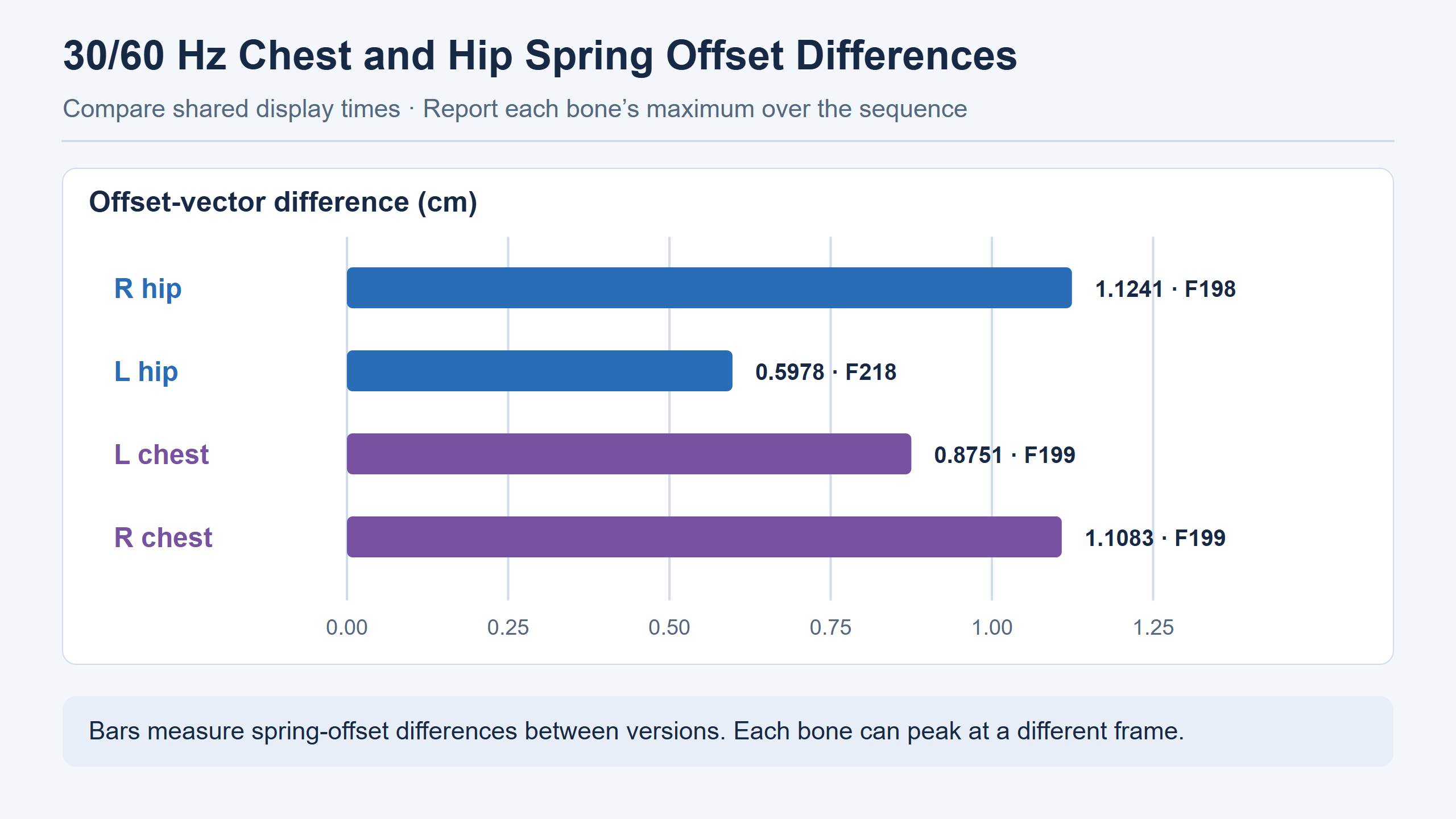
The chest spring’s 1 cm cap constrains the target-relative offset within one version. The right-chest value of 1.1083 cm compares the offset vectors from the 30 Hz and 60 Hz versions. They measure different quantities. The 1 cm cap limits the offset length within one version relative to that version’s target at a given time. The table measures the difference between two versions’ offset vectors. If A offsets 0.6 cm along component +X and B offsets 0.6 cm along −X, both satisfy a 1 cm cap, but they are 1.2 cm apart. With a shared target and basis, two offsets capped at 1 cm can differ by up to 2 cm. The 2 cm value is a theoretical bound for a shared target and coordinate basis. The measured offsets need not be collinear or point in opposite directions.
P95 interframe displacement instead measures motion within one version. It takes one bone’s positional change from frame n to n+1 within one version, then computes the segment’s 95th percentile. This describes a high but commonly observed interframe displacement, not the maximum. The target also moves, so a target-relative spring cap cannot bound total interframe bone motion. Turns, torso lean, and clip phase can all change that statistic. First identify whether a table compares versions at one frame or frames within one version, and then check its coordinate space.
| Region | Display frame of maximum offset difference | 30/60 Hz offset-vector difference |
|---|---|---|
| Right hip helper | 198 | 1.1241 cm |
| Left hip helper | 218 | 0.5978 cm |
| Left chest helper | 199 | 0.8751 cm |
| Right chest helper | 199 | 1.1083 cm |
These are spring-offset differences for four bones in the default-combat candidate. Their maxima can occur on different frames. Adding them does not give a body difference at frame 199, and they cannot be converted into maximum mesh displacement. A skinned vertex can be influenced by several bone transforms and weights, while chest rotation and correction add further effects. Mesh measurements require a separate comparison with matching vertex IDs, LOD, binding, and complete skinning palettes.
Comparing steady gaits and animation transitions
Walking and running each retain two cycles from the continuously solved steady segment. Walking uses a frontal chest view and a rear-quarter hip view; running uses a side chest view. Both cameras in each group start at the same source frame and can be played or paused independently.
Walking loop
Show the walking loop at half speed
Running loop
Show the running loop at half speed
The source cache is solved at 60 Hz, and every second frame is exported at 30 FPS. Walking covers source interval [144, 288), with cycle two starting at 216. Running covers [160, 240), with cycle two starting at 200. Half speed extends display duration. The wraparound image difference is within each clip’s range of adjacent-frame differences. The running side-chest view is closest to that upper bound, so a small loop-boundary change may remain visible.
The gait report separates seven intervals. The table lists the maximum observed spring-offset difference for either hip bone and either chest bone within each interval, rounded to the report’s precision. A transition peak does not describe the full sequence, and a still image cannot establish response speed. The paired images locate useful slow-motion inspection points; frame numbers lead back to the calculation records.
| Action | Display frames, inclusive | Hip peak | Chest peak |
|---|---|---|---|
| Walk | 1–36 | 0.33 cm(21) | 0.28 cm(9) |
| Walk to run | 37–58 | 0.39 cm(58) | 0.65 cm(48) |
| Run | 59–112 | 0.39 cm(68) | 0.43 cm(99) |
| Run to sprint | 113–133 | 0.56 cm(117) | 0.42 cm(117) |
| Sprint | 134–179 | 0.35 cm(134) | 0.27 cm(178) |
| Release sprint input | 180–189 | 0.20 cm(181) | 0.33 cm(186) |
| Sprint-stop candidate | 190–280 | 1.12 cm(198) | 1.11 cm(199) |
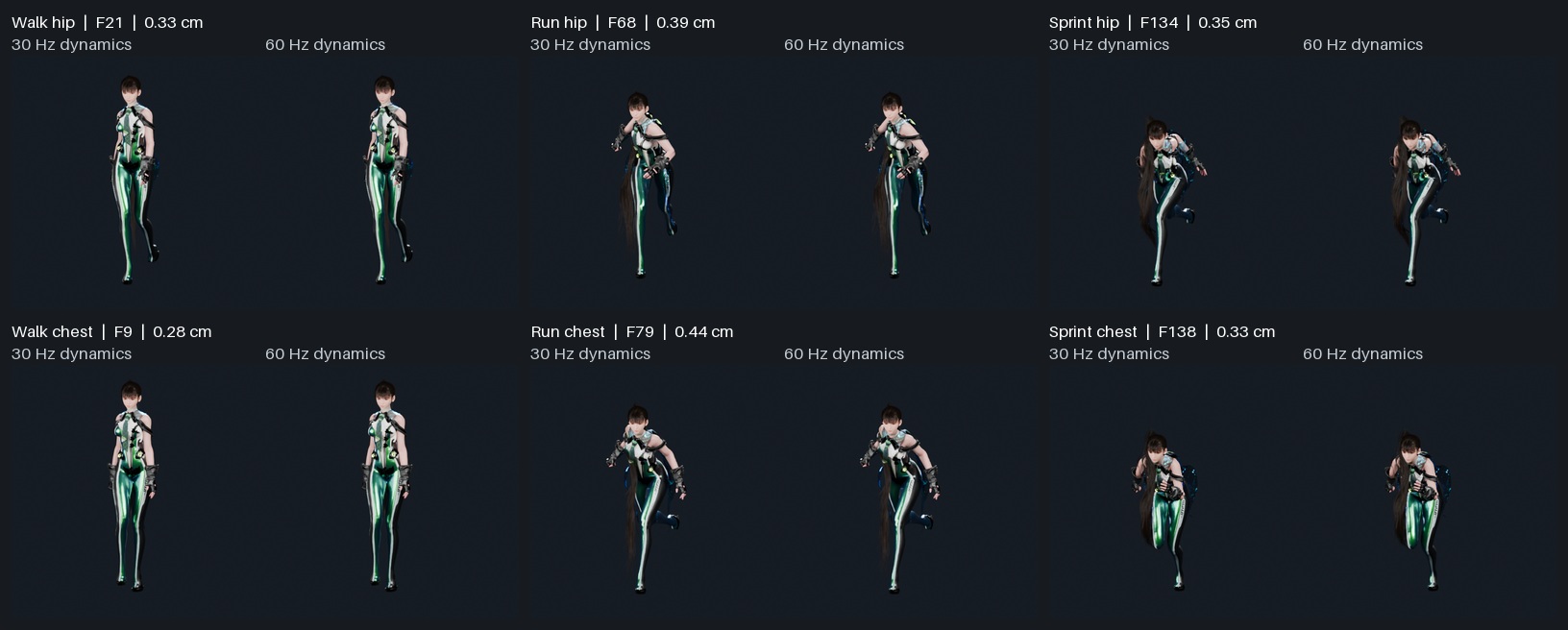
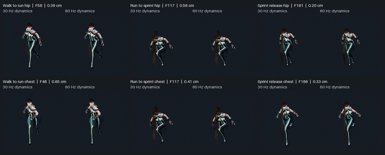
Frame 117 falls in the run-to-sprint segment and is also that interval’s hip and chest peak, making it useful for examining both groups’ response to the changed base pose. Frames 198 and 199 are adjacent but distinct, highlighting the right hip and right chest respectively. The left hip’s maximum occurs later at 218. Applying one peak frame to every node would imply shared integration state. The records calculate each bone separately; its own target and history determine the peak.
Other tables report pelvis-space position differences and interframe step differences in that space. Pelvis space reveals motion relative to a torso reference and reduces the contribution of overall pelvis translation. Spring offset remains the integrated result relative to the target. These values may be close or may differ because of rotation, downstream correction, or the measured object. Specify whether a figure shows offset, position, or a time difference. A label such as maximum error alone loses that distinction.
Kernel reproduction error and input-rate differences
The default-combat 30 Hz cache differs from original-instruction replay with specified inputs by a maximum coordinate component of about 0.000092 cm. At selected marker frames in the 60 Hz A/B report, original SpringBone replay has a maximum component difference of 0.000033 cm. These comparisons fix inputs and timing before comparing reconstructed and original calculations. By contrast, the right hip’s 1.1241 cm at frame 198 is a motion difference between configurations. The first tests kernel agreement for specified inputs; the second examines changed external-update timing.
Historical reports use narrower comparison ranges and different error bounds. State the candidate version, input frequency, full-sequence or marker-frame coverage, and compared components together. Two small values do not justify choosing the smaller as a general in-game accuracy claim. Original-instruction replay, offline-cache comparison, and reopened Blender results retain their respective measurement scopes.
Separating base-animation and procedural displacement
The archived body build includes outputs named source、hips、constrained、chest、full、no_spring_full. The names identify comparison stages. In particular, hips is a diagnostic that exports only hip-bone results. File order does not establish execution order or show that one diagnostic output becomes the input to the next solver stage. Choose the stage to inspect before selecting its before-and-after poses.
| Question | Stages to compare | Required context |
|---|---|---|
| How much motion comes from source animation? | Source pose and final pose for the same segment | Same bone, frame interval, and coordinate space |
| What did the hip spring directly change? | The isolated hip-bone diagnostic output | Bone name, target translation, and integrated offset |
| What did the chest constraint change? | Source and constrained poses | Same-side target orientation, reference offset, and local axes after writeback |
| How does adding the spring change the final pose? | Full branch versus the full branch without the spring | BtoB remains active; upstream changes can alter its inputs |
| How is correction written into the skeleton? | Post-spring pose and final pose | Upper-limb distances and local translation/scale before and after correction |
Run-to-sprint provides a direct counterexample to attributing all visible motion to physics. In the default-combat layered records, final interframe displacement P95 is 6.07/9.04 cm for hip/chest, while the decoded source pose already measures 7.25/9.16 cm. In the final footage alone, the strong local movement can look like a large added physics response. Comparing source and final poses shows that the animation already supplies substantial displacement; the solved result is slightly smaller under these statistics.
Steady-gait motion also does not simply increase uniformly with speed. For walk/run/sprint, final interframe P95 is 1.33/2.76/3.18 cm at the hips and 1.08/3.00/2.68 cm at the chest. Chest and hip rank running versus sprinting differently. Compare by node, stage, and measurement definition. Scaling chest and hip amplitudes by one gait-speed value cannot reproduce the candidate’s target curves and downstream solution.
Vector decomposition of local displacement
To explain a final bone’s displacement at a transition, express each stage’s change over the same frame interval as a vector. Let S₀ and S₁ be source positions and F₀ and F₁ final positions. Source displacement is ΔS = S₁ − S₀; final displacement is ΔF = F₁ − F₀. Their difference measures the final branch’s change relative to the source. For actual sequential stages, compute each stage’s displacement and then subtract adjacent stages’ vectors. Outputs from independent toggle tests are not successive stages of the same calculation and cannot be summed as intermediate contributions.
When ΔF is nonzero, define the final motion direction as u = ΔF / |ΔF|. Project each contribution onto u and retain its sign. Positive values add motion along the final direction; negative values cancel it. Perpendicular components change direction without adding length along u. If ΔF is near zero, the unit direction is unstable, so retain the original vectors or skip directional attribution. Adding displacement magnitudes overestimates the result for this reason.
For a 2D example, source displacement is (4, 0) cm and one downstream contribution is (−1, 2) cm. Final displacement is (3, 2), about 3.61 cm long. Adding the two magnitudes gives about 6.24 cm. Projection onto the final direction assigns about 3.33 cm to the source and 0.28 cm to the added stage, totaling about 3.61 cm. This illustrates attribution; engineering records still need the coordinate space, frame interval, and compared stage outputs.
Animation input and transition timing during a sprint stop
We have examined how the spring uses target position x. To explain the stop’s largest offset difference, we must also trace x to its source. Each animation instance is sampled on its own clock, and the resulting pose is exported at 280 display times. Display frames set capture times. A clip’s sampling cursor depends on its start phase, playback advance, and weight history. Multiplying a display-frame number by one clip’s sample interval misaligns clips with different lengths, weights, and entry times.
Show the HD normal-speed version
In this offline example, frame 190 registers the stop candidate, and frame 191 first advances its sampling cursor. With display time t = (n − 1)/30, these are 6.30 s and approximately 6.33 s. Registration and cursor advancement occur at different evaluation times. Frame 190 retains the previous pose, so time zero of the new clip cannot directly stand for that frame’s output. Frames 191–194 reveal how the player mixes outgoing and incoming motion.
Display time, animation sample time, and blend weights
The first layer is base locomotion. Speed and other parameters enter the source asset’s RunTilt gait-blending grid, which selects contributing gait animations and computes their target blend weights. The source assets establish a sample-weight interpolation rate of 4/s for that grid. Approaching a new target takes multiple updates, so a character-input or target-weight change can initially retain the previous blended result.
The second layer is clip sampling. As weights change, each sample advances through its own normalized clock. Clips have their own effective lengths and starting phases. Driving both with elapsed video time changes foot phase and body-target trajectories. Blending happens after the corresponding QTS samples are obtained. An animation-state name identifies an active path; player records establish which samples actually contributed and at what weights.
The third layer is the character overlay. The sprint-stop layer accepts a new clip while the outgoing clip can still contribute inside the player. The character layer can inherit its active weight, even displaying full weight, but that only describes its use of the player’s output. The player can still output a blend of old and new animation. The recovered 4/s rate belongs to the first layer and cannot predict the third layer’s transition duration.
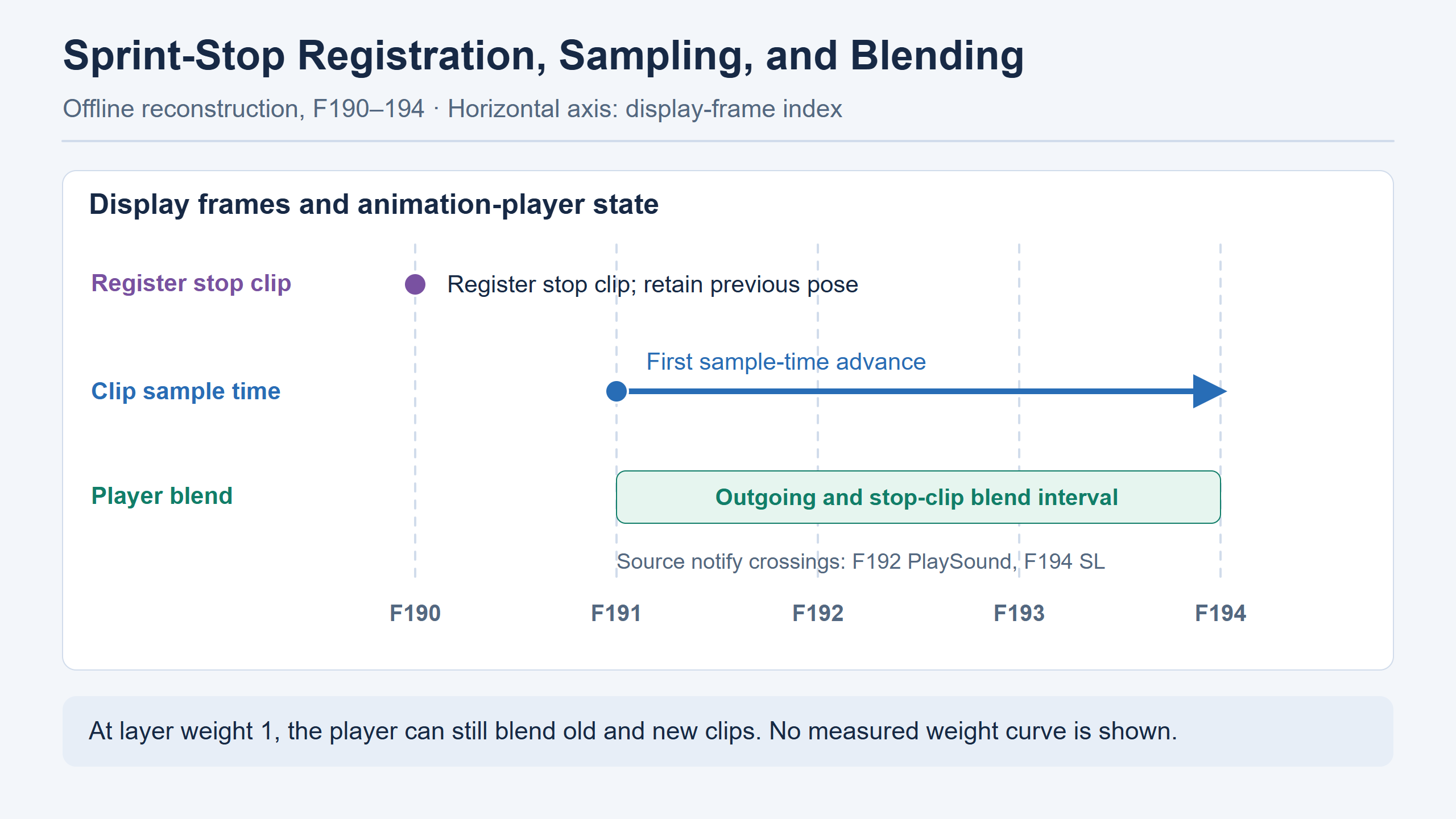
For example, suppose the player outputs 70% of the old pose and 30% of the new pose. A character-layer weight of 1 uses that output in full, including the retained 70% outgoing contribution. Actual rotation blending follows the pose representation and engine convention. These percentages only explain the relationship between layers; they do not reconstruct frame 191’s weights. The shared records establish transition identity and timing, but do not supply the original per-frame weight curve.
Offline notify timing and runtime dispatch
In the same stop candidate, display frames 192, 194, and 231 first cross the source times of PlaySound, SL, and WR respectively. These frame numbers align the in-place video with sample records. Actual in-game dispatch also depends on runtime notify scanning, animation update order, and playback instances. A crossed threshold may be dispatched in another stage or filtered by weight and instance lifetime. The material locates offline crossings but supplies no in-game dispatch trace for this clip.
Likewise, the diagnostic stop distance of 65.72 cm comes from a test trajectory replay. The Blender footage keeps the character at a fixed presentation position for pose comparison. It does not record world travel or verify in-game foot contact. Measuring against its background would describe only the offline presentation. Linking displacement and pose requires root transforms, world-space sole positions, and contact conditions from the same trajectory replay.
Tracing spring differences from the source pose
If two stop implementations already differ at frame 190, compare source sampling, character-layer weights, and parent component matrices first. There is no basis yet for attributing that difference to spring substeps. If source and constrained poses match at common display times but centimeter-scale offsets appear at frames 198–199, inspect preceding midpoint inputs, remainder, and velocity history. Work backward from the first differing stage to narrow the cause.
An animation-segment boundary is not a solver-reset boundary. Frames 180–189 cover input release and the offline exit from sprinting. At frame 190, helper bones continue using spring state from the preceding motion. Solving frames 190–280 alone from a freshly initialized pose discards that velocity. The half-speed stop is extracted from continuous results. Slow playback extends each frame’s display duration without reevaluating the solver.
This is why transition analysis starts with the full sequence before cutting to close-ups. An isolated running clip shows steady gait but cannot test a stop after accumulated motion. At 30 FPS, frames 198 and 199 are only about 33 ms apart. Use source numbering or per-frame records to find them; a browser timestamp rounded to six seconds cannot reliably distinguish neighboring samples.
Left-foot stop correction and downstream pose input
In the chest/hip frequency experiment, both branches have identical ankle and toe matrices at shared display times. This controls the tested foot chains for that experiment. A separate diagnostic explicitly modifies the left leg to address sole placement during stopping. One changes body-dynamics input timing; the other changes the final left-leg pose. The latter changes cloth and hair collision inputs and provides the next article’s starting point.
Show the HD half-speed version
The sole diagnostic uses sole vertices from the original mesh at its highest level of detail (LOD0). Ground-relative height measures the deepest penetration. Here, horizontal residual means the horizontal displacement of near-ground sole vertices between two frames, used to inspect foot sliding. The measurement first selects vertices near the ground in both consecutive frames, then measures their horizontal movement. At frame 193, the left sole reaches approximately −8.26 cm, with no vertices within the ±2 cm near-ground band. Reporting zero residual would confuse an empty sample set with zero displacement. Record sample count alongside the measurement and explicitly mark an empty set.
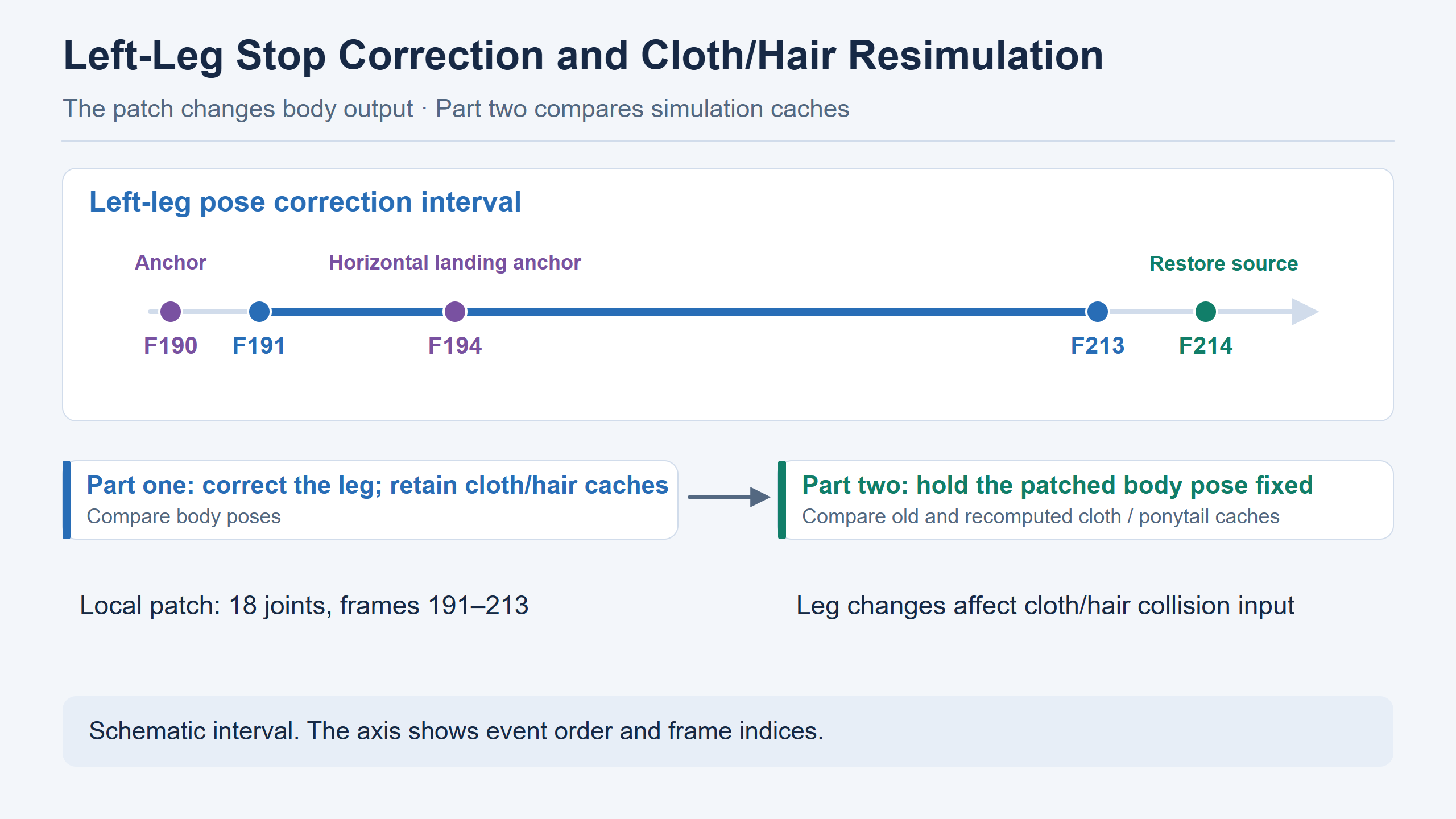
The patch retains frame 194’s horizontal landing target and tests a swing arc with an additional 3 cm of clearance. It rewrites final local matrices for 18 joints only within frames 191–213, returning to the original pose at frame 214. Anchors define the correction, the patch interval determines rewritten frames, and the restoration point returns to source motion. Using frame 194 as an anchor does not mean all its local matrices stay unchanged, nor does a 24-frame surrounding interval define the patch window. This is an offline diagnostic patch, not established in-game IK.
The patch also exposes the handoff between pose and simulation caches. This article’s short comparison retains the original cloth and ponytail caches on the patched side so the body change can be inspected first. The visible surfaces at those timestamps still correspond to the old input, changing their relationship to the corrected leg. The next article fixes the patched body pose and compares old and recomputed caches from the same camera. Even after body matrices return to their original values, surface particles can retain different histories. This resembles cross-segment spring history, although the states and solvers differ.
Measuring sole penetration and sliding
For helper-bone evaluation, LOD0 sole vertices can serve as controls expected to remain unaffected. Matching foot chains and shoe-surface values at both input rates show that the comparison has not also modified the legs. Foot correction needs different metrics: deepest penetration, near-ground sample count, horizontal residual, and contact continuity. A zero difference between versions does not establish penetration-free feet; both can penetrate equally.
A foot patch also needs an explicit anchor definition. Preserving a horizontal landing target and raising a swing arc can coexist: one constrains the endpoint, the other changes height along the trajectory. Moving the whole character vertically would obscure the left-leg solver’s contribution. Compare the leg from the same camera and retain the same vertex set. The chest/hip comparisons follow the same principle: matched pelvis pose, parent transforms, and sample time give the local helper-bone change a clear interpretation.
Bone writeback and original-instruction comparison
Verification has two levels. First check matrix representations between stages, including bone indices, local transforms, and skeletal submission. Then check state evolution through continuous spring and correction updates. A matrix-layout mistake can affect one bone on one side, whereas an update-order mistake can leave the first few frames apparently correct.
For source、hips、constrained and chest, the project checks matrix-to-QTS conversion, passage through original Rig I/O, and conversion back to matrices. This tests a stage’s round trip through the representation used by the original interface. Shared indices must refer to the same nodes, and local scale signs must survive decomposition. Looking only at the mesh can hide errors behind other transforms. A changed local axis might leave a child close to its original position in one frame but send it in the wrong direction when rotation changes next frame.
For full and no_spring_full, the project executes BtoB continuously and retains its accumulator for the sequence. Evaluating frame 199 alone without the preceding 198 frames changes that history. A minimal replay can begin with a recorded complete state and supply the remaining inputs in order. Without that state, solve from the beginning of the same sequence. Both spring-on and spring-off branches need consistent initialization and warm-up.
Stage-by-stage error checks from source animation to final pose
Consider the right-chest diagnostic. Fix the sequence, character configuration, and 30/60 Hz conditions. Decide whether the question is frame 199’s frequency difference or a component difference between offline and original-instruction results at one frequency. This determines the compared columns. Different-frequency inputs sent to two kernels cannot establish an implementation error.
Then align display times and solver records. Frame 199 corresponds to (199 − 1)/30 = 6.60 s. The 60 Hz version has processed extra intermediate inputs before reaching it. Read target and p together; retain pre-clamp results if available. For rotation, record the constraint and parent chain separately rather than labeling chest orientation changes as SpringBone translation error.
| Checkpoint | Record | Likely diagnostic area |
|---|---|---|
| Source sampling | Clip identity, local sample time, current weight, local QTS | Animation phase, segment entry, and inherited weights |
| Forward kinematics | Target/helper parent indices and component matrices | Bone index, parent chain, and reference space |
| Chest constraint | Reference target rotation, reference offset, and current target rotation | Wrong same-side target, multiplication order, or scale included in rotation |
| Spring substep | dt, remainder, x, p, v, history, and limits | Equality boundaries, reset, and history-update order |
| BtoB | Upper-limb distances, accumulated correction, and final local matrix | Input space, side-specific coefficients, and local scale |
| Blender display | Corresponding skeleton version, camera, frame, and surface cache | Animation branch, sampling time, or stale surface cache |
If replay with identical inputs matches p and v but the final image differs, inspect local writeback and Blender’s transform interpretation. If the discrepancy exists before the spring, trace the target’s source stage. A difference in the first substep can be attributed to kernel calculations only when inputs, histories, and branches match. This avoids repeatedly adjusting damping against mismatched timing until one video happens to align.
What assets, instruction replays, and renders can verify
Original animation assets establish tracks, notifies, and sample configuration. Static data alone usually cannot establish an equipment overlay’s active weight in every frame. Original executable instructions with specified inputs reveal comparison operators, update order, and numerical results. Continuous offline solving selects an input trajectory and timeline to connect recovered stages. Blender displays the result. The video cannot reveal an unsubmitted animation-graph path or visually separate near-identical bone components.
A configuration reference with weight 0.4, an earlier experiment that used 0.4, and a current sequence with zero Type1 weight are compatible observations. They require the asset table, earlier experiment record, and current active-weight log respectively. Similarly, a specified-input SpringBone replay below one ten-thousandth of a centimeter establishes agreement for tested calculations, while in-game inputs, full graph order, and real-time skinning submission remain separate checks. Measurements in this article retain their compared objects and versions.
Full-body pairs show continuous motion and transitions. Subcentimeter bone differences require close-ups and transform records. The added technical videos project same-frame data onto the render: cyan targets, amber spring outputs, and axes following the parent’s local basis. Chest markers are sampled before BtoB, while final skinning includes later correction. These show results at displayed sample times; substep integration still requires numerical records. The SVG bone and axis examples explain calculations, with actual positions supplied by the source skeleton and delivered data.
Independent checks of coordinate transforms and state history
Before porting, a target-and-spring-state test can exclude the skeleton, animation, and rendering. Supply horizontal targets and a matching initial position to one bone, execute several external updates, and record each substep. Translate all targets and initial positions by the same amount while retaining velocity, history, clocks, and parameters. Under the described update, x − p, restoring terms, and damping terms remain unchanged. Output positions should differ by that translation, while target-relative offsets match. Allow float32 rounding, particularly when small centimeter offsets sit on very large coordinates. This is a suggested teaching check; the handoff does not report having run it.
Then connect the teaching input to a local track with parent rotation. At +90° around Z, the component displacement must pass through the current parent’s inverse. Recompose the written result with that same parent to check that component displacement retains the requested direction. This isolates space conversion with a fixed parent chain and target. Using the previous frame’s parent inverse can produce a small local difference that rotates with the new parent chain. A single-frame writeback check is useful before investigating continuous spring jitter during turns.
Another check copies a complete state at a chosen position and velocity during the same target sequence. One copy retains the velocity ring and remainder, while the other retains only p and v. Continue with identical targets. Before new velocities replace every history slot, the averages can differ. A remainder near the substep boundary can also change the number of iterations despite identical dt. A restart snapshot therefore needs buffer contents, indices, and unprocessed time. Retaining only the visible pose can reproduce the first frame while subsequent recovery diverges.
The chest constraint can be tested without the spring. Set the current same-side target rotation to its reference rotation. The helper’s new component rotation should then recover its own reference rotation, as R_ref_target and its inverse cancel. Change the target orientation and inspect whether the relative relationship is preserved. Compare component translations before and after as a separate control for rotation-only modification. Check all three scale values too; rotation quaternions alone cannot establish preservation through decomposition. Each output—orientation, translation, and scale—needs its own check.
An independent BtoB test can begin with upper-limb geometry. Fix a chest pose and change only one forearm’s component-space input. Track distance, branch selection, target correction, accumulator, and modified local-matrix elements. Rotate the parent and check which axes serve component-distance calculations and local X writeback. Moving the hand in world space alone does not establish a shorter distance because pose, component transform, and the target can all change. Test both sides with their respective coefficients and conventions. The handoff establishes dependencies and accumulation; complete coefficients need checking against the developer’s implementation.
These checks locate timing, coordinate, and correction-input issues separately. Return them to the same full-character sequence for regression and trace the first divergence. If animation targets and spring states agree but BtoB accumulation differs, inspect arm distances and dt. If bone matrices agree but the silhouette differs, inspect binding, skinning weights, and the mesh. The next article follows those body poses into cloth and ponytail motion.
Reproduction workflow and source entry points
Begin with the archived sequence inputs. Check source animation and active weights for the same sequence ID, then build the 30 and 60 Hz body caches. The 60 Hz build reads preceding weights and the baseline manifest, supplies intermediate poses, and updates body dynamics continuously. Finally export at matching display times. These dependencies matter more than script paths. Skipping upstream pose conditions or reading the wrong weight history can compare different body inputs even when both videos have identical frame counts.
The following entry points are grouped by responsibility. General script paths are retained, while character-specific scripts are identified by purpose. The article materials include analysis, comparison tables, images, and videos. The complete project remains with the development workspace.
| Project entry point | Purpose |
|---|---|
scripts/audit_combined_ground_tracking.py |
Audit combined animation and sole diagnostics; locate the stop interval |
scripts/audit_native_sprint_stop_clock.py、scripts/audit_native_sprint_stop_overlay_overlap.py |
Check stop cursor advancement and outgoing/incoming clip overlap |
scripts/audit_native_battle_sample_weights.py, plus the default-combat pose-weight audit |
Check active gait-sample and equipment-overlay weights |
scripts/build_locomotion_sequence_body.py、scripts/build_idle_transition_body.py |
Build continuous body poses and dynamics outputs |
runtime/secondary_motion.py、scripts/native_spring_kernel.py、scripts/native_spring_pose.py |
Compare spring steps, original instructions, and pose inputs |
| Left-leg diagnostic and stop-patch build scripts | Diagnose the stopping left leg and generate isolated patched poses |
Compare source data and body manifests under the same configuration first. Default-combat and 60 Hz builds both need matching upstream products. Manifest hashes identify exact files. The article uses descriptive names such as source animation, current combat candidate, and 30/60 Hz comparison so readers can identify the columns before tracing precise inputs. Video decoding and hash checks establish delivery integrity and frame order.
For a UE port, first place each pose stage in the evaluation pipeline. The component-space spring needs its base pose ready, and output timing must match later constraints and skinning reads. Then establish clock inputs, history across state changes, and handling of long intervals when a character stops updating. These are integration checks inferred from the offline result; the handoff contains no current in-game Tick or scheduling trace. The Blender footage does not establish completed UE integration.
Additional animation clips
These half-speed clips come from the same 60 Hz body-dynamics candidate and isolate individual motion stages. Use them to revisit body pose and timing. Close-ups, the full frequency comparison, sprint stop, and left-leg patch appear in their corresponding sections.
Show the HD normal-speed version
Show the HD normal-speed version
Show the HD normal-speed version
Show the HD normal-speed version
Show the HD normal-speed version
Show the HD normal-speed version
From body pose to secondary motion
Returning to the opening stop, we can now trace the local changes through their update order. Base animation changes the body and arms. The chest rotation constraint retains the reference orientation relationship. Translation springs receive new component-space targets while carrying earlier positions, velocities, and time remainder. BtoB then adjusts the chest’s local transform using current arm distances. Together these stages produce the pose supplied to skinning.
Walking and running loops show the response to periodic targets. Stopping combines target deceleration, animation blending, and inherited state. Identical target positions can yield different outputs under different velocity histories. Playing a clip in isolation and reinitializing the spring changes that history, so transition reproduction needs the preceding motion too.
The implementation needs spatial and temporal records together. Targets, integrated positions, and arm distances use the agreed component space, with the current parent matrix used for local writeback. Base-pose sampling, external submissions, spring substeps, and display frames each have their own timing role. The formulas, pseudocode, and technical overlays keep these relationships visible so that the first discrepancy can be located at a particular stage.
The continuous sequence, frequency comparison, spring traces, and BtoB toggles provide the corresponding checks. In an engine, repeat them within actual animation evaluation, covering recovery after paused updates, state transitions, and downstream pose reads. Saving each stage’s transforms alongside same-frame footage makes later differences traceable to individual calculations.
The next article begins with this final body pose. Cloth and ponytail systems use it to update deformation, constraint anchors, and collision input. A small body correction can therefore alter their trajectories over subsequent frames. We will retain the left-leg stop patch and compare the old cache with a recomputed result, following the change from body bones to visible cloth and hair.
AI collaboration retrospective
AI supported the organization of handoff material, placement of continuous and close-up comparisons, mechanism diagrams, and bilingual editing. Animation and solver parameters were grounded in the developer-supplied assets, transform records, and original-instruction replays. Spring traces, steady gait loops, and an independent BtoB toggle were added during production to connect the described calculation stages with visible results.
The revisions also exposed gaps in turning engineering material into an article. Early full-body previews were only 480×480 and lost useful detail when displayed at article width. The first schematic figures did not communicate body proportions and coordinate transforms clearly, and some code and table formatting missed the established site rules. Following the user’s feedback, the development side rendered HD footage and additional close-ups. The article diagrams and formula annotations were revised, then checked against the existing blog standards.
The practical lesson is to tie every observation to suitable footage and data. Full-body motion needs its transitions preserved, close-ups need a camera that reveals the relevant movement, and algorithm comparisons need controlled inputs and initial state. These conditions and the existing writing rules should be checked before translation and layout. Diagrams, transform records, and continuous footage together let readers trace the implementation.